
Microsoft Excel is one of the most powerful spreadsheet tools, with an impressive collection of built-in tools and features. In this article, you’ll learn how powerful Excel formulas and conditional formatting can be, with three useful examples.
Digging Into Microsoft Excel
We’ve covered a number of different ways to make better use of Excel, such as using it to create your own calendar template or using it as a project management tool.
Much of the power lies behind the Excel formulas and rules that you can write to manipulate data and information automatically, regardless of what data you insert into the spreadsheet.
Let’s dig into how you can use formulas and other tools to make better use of Microsoft Excel.
Conditional Formatting With Formulas
One of the tools that people don’t use often enough is Conditional Formatting. If you’re looking for more advanced information on conditional formatting in Microsoft Excel, make sure to check out Sandy’s article on formatting data in Microsoft Excel with conditional formatting.
With the use of Excel formulas, rules, or just a few really simple settings, you can transform a spreadsheet into an automated dashboard.
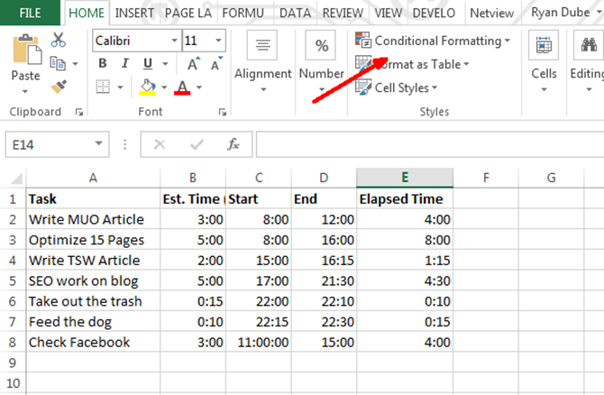
To get to Conditional Formatting, you just click on the Home tab, and click on the Conditional Formatting toolbar icon.
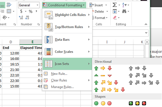
Under Conditional Formatting, there are a lot of options. Most of these are beyond the scope of this particular article, but the majority of them are about highlighting, coloring or shading cells based on the data within that cell.
This is probably the most common use of conditional formatting—things like turning a cell red using less-than or greater-than formulas. Learn more about how to use IF statements in Excel.
One of the lesser used conditional formatting tools is the Icon Sets option, which offers a great set of icons you can use to turn an Excel data cell into a dashboard display icon.
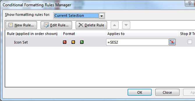
When you click on Manage Rules, it’ll take you to the Conditional Formatting Rules Manager.
Depending on the data you selected before choosing the icon set, you’ll see the cell indicated in the Manager window, with the icon set you just chose.
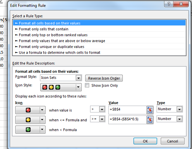
When you click on Edit Rule, you’ll see the dialog where the magic happens.
This is where you can create the logical formula and equations that will display the dashboard icon you want.
This example dashboard will show time spent on different tasks versus budgeted time. If you go over half the budget, a yellow light will display. If you’re completely over budget, it’ll go red.
As you can see, this dashboard shows that time budgeting isn’t successful.
Almost half of the time is spent way over the budgeted amounts.
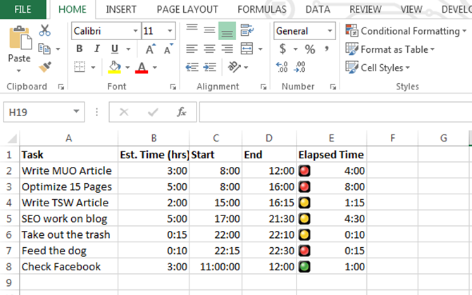
Time to refocus and better manage your time!
1. Using the VLookup Function
If you’d like to use more advanced Microsoft Excel functions, then here’s another one for you.
You’re probably familiar with the VLookup function, which lets you search through a list for a particular item in one column, and return the data from a different column in the same row as that item.
Unfortunately, the function requires that the item you’re searching for in the list is in the left column, and the data that you’re looking for is on the right, but what if they’re switched?
In the example below, what if I want to find the Task that I performed on 6/25/2018 from the following data?
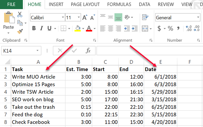
In this case, you’re searching through values on the right, and you want to return the corresponding value on the left – opposite the way VLookup normally works.
If you read Microsoft Excel pro-user forums you’ll find a lot of people saying this isn’t possible with VLookup, and that you have to use a combination of Index and Match functions to do this. That’s not entirely true.
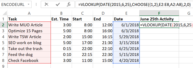
You can get VLookup to work this way by nesting a CHOOSE function into it. In this case, the Excel formula would look like this:
"=VLOOKUP(DATE(2018,6,25),CHOOSE({1,2},E2:E8,A2:A8),2,0)"
What this function means is that you want to find the date 6/25/2013 in the lookup list, and then return the corresponding value from the column index.
In this case, you’ll notice that the column index is “2”, but as you can see the column in the table above is actually 1, right?
That’s true, but what you’re doing with the “CHOOSE” function is manipulating the two fields.
You’re assigning reference “index” numbers to ranges of data – assigning the dates to index number 1 and the tasks to index number 2.
So, when you type “2” in the VLookup function, you’re actually referring to Index number 2 in the CHOOSE function. Cool, right?
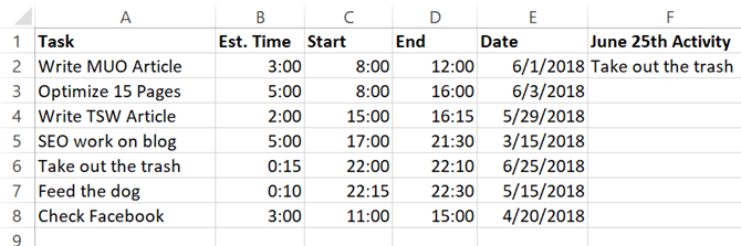
So, now the VLookup uses the Date column and returns the data from the Task column, even though Task is on the left.
Now that you know this little tidbit, just imagine what else you can do!
If you’re trying to do other advanced data lookup tasks, be sure to check out Dann’s full article on finding data in Excel using lookup functions.
2. Nested Formula to Parse Strings
Here’s one more crazy Excel formula for you.
There may be cases where you either import data into Microsoft Excel from an outside source consisting of a string of delimited data.
Once you bring in the data, you want to parse that data out into the individual components. Here’s an example of name, address and phone number information delimited by the “;” character.
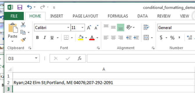
Here’s how you can parse this information using an Excel formula (see if you can mentally follow along with this insanity):
For the first field, to extract the leftmost item (the person’s name), you would simply use a LEFT function in the formula.
"=LEFT(A2,FIND(";",A2,1)-1)"
Here’s how this logic works:
- Searches the text string from A2
- Finds the “;” delimiter symbol
- Subtracts one for the proper location of the end of that string section
- Grabs the leftmost text to that point
In this case, the leftmost text is “Ryan”. Mission accomplished.
3. Nested Formula in Excel
But what about the other sections?
There may be easier ways to do this, but since we want to try and create the craziest Nested Excel formula possible (that actually works), we’re going to use a unique approach.
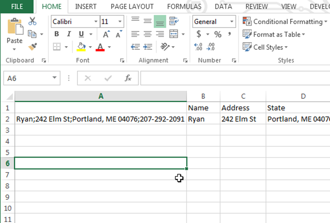
To extract the parts on the right, you need to nest multiple RIGHT functions to grab the section of text up until that first “;” symbol, and perform the LEFT function on it again. Here’s what that looks like for extracting the street number part of the address.
"=LEFT((RIGHT(A2,LEN(A2)-FIND(";",A2))),FIND(";",(RIGHT(A2,LEN(A2)-FIND(";",A2))),1)-1)"
It looks crazy, but it’s not hard to piece together. All I did is took this function:
RIGHT(A2,LEN(A2)-FIND(";",A2))
And inserted it into every place in the LEFT function above where there’s an “A2”.
This correctly extracts the second section of the string.
Each subsequent section of the string needs another nest created. So now you just take the crazy “RIGHT” equation you had created for the last section, and then pass that into a new RIGHT formula with the previous RIGHT formula pasted into itself wherever you see “A2”. Here’s what that looks like.
(RIGHT((RIGHT(A2,LEN(A2)-FIND(";",A2))),LEN((RIGHT(A2,LEN(A2)-FIND(";",A2))))-FIND(";",(RIGHT(A2,LEN(A2)-FIND(";",A2))))))
Then you take THAT formula, and place it into the original LEFT formula wherever there’s an “A2”.
The final mind-bending formula looks like this:
"=LEFT((RIGHT((RIGHT(A2,LEN(A2)-FIND(";",A2))),LEN((RIGHT(A2,LEN(A2)-FIND(";",A2))))-FIND(";",(RIGHT(A2,LEN(A2)-FIND(";",A2)))))),FIND(";",(RIGHT((RIGHT(A2,LEN(A2)-FIND(";",A2))),LEN((RIGHT(A2,LEN(A2)-FIND(";",A2))))-FIND(";",(RIGHT(A2,LEN(A2)-FIND(";",A2)))))),1)-1)"
That formula correctly extracts “Portland, ME 04076” out of the original string.
To extract the next section, repeat the above process all over again.
Your Excel formulas can get really loopy, but all you’re doing is cutting and pasting long formulas into itself, make long nests that actually work.
Yes, this meets the requirement for “crazy”. But let’s be honest, there is a much simpler way to accomplish the same thing with one function.
Just select the column with the delimited data, and then under the Data menu item, select Text to Columns.
This will bring up a window where you can split the string by any delimiter you want.
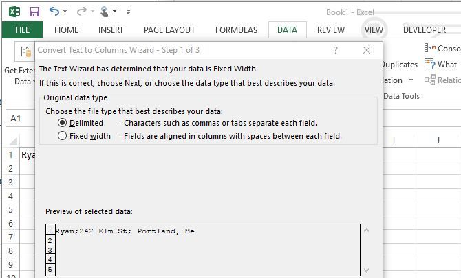
In a couple of clicks you can do the same thing as that crazy formula above… but where’s the fun in that?
Getting Crazy With Microsoft Excel
So there you have it. The above formulas prove just how over-the-top a person can get when creating Microsoft Excel formulas to accomplish certain tasks.
Sometimes those Excel formulas aren’t actually the easiest (or best) way to accomplish things. Most programmers will tell you to keep it simple, and that’s as true with Excel formulas as anything else.
If you really want to get serious with using Excel, you’ll want to read through our beginner’s guide to using Microsoft Excel. It has everything you need to start boosting your productivity with Excel.
Read the full article: 3 Crazy Excel Formulas That Do Amazing Things
Read Full Article
No comments:
Post a Comment