If you have a lot of data in a worksheet, or you’re working on a small screen, you can hide data on your spreadsheet to make it easier to view and analyze your data.
Today we’ll show you how to conceal different areas on your worksheets and hide the data.
How to Hide and Unhide Overflow Text
When you type text in a cell, and the text is wider than the cell, the text overflows into the adjacent cells in the row. If there is any text in the adjacent cell, the text in the first cell is blocked by the text in the adjacent cell.
You can solve this by having the text wrap in the first cell. But that increases the height of the entire row.
If you don’t want to show the overflow text, even when there is nothing in the adjacent cells, you can hide the overflow text.
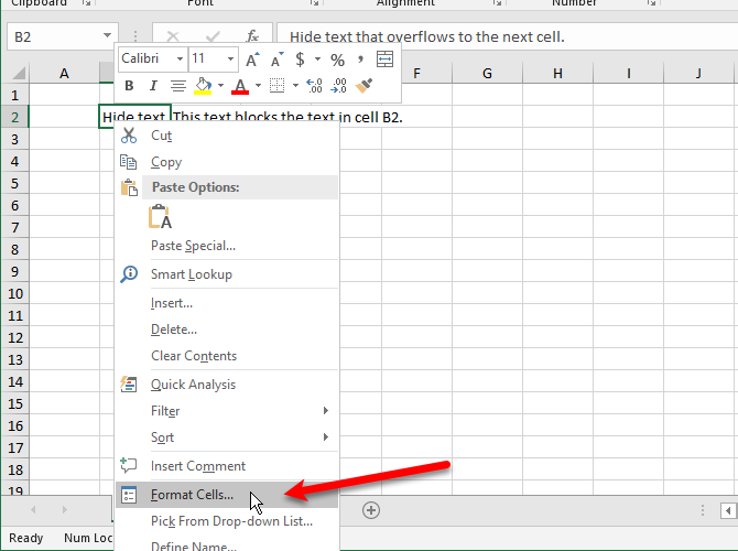
Select the cell containing the text that’s overflowing and do one of the following:
- Right-click on the selected cell(s) and select Format Cells.
- Press Ctrl + 1.
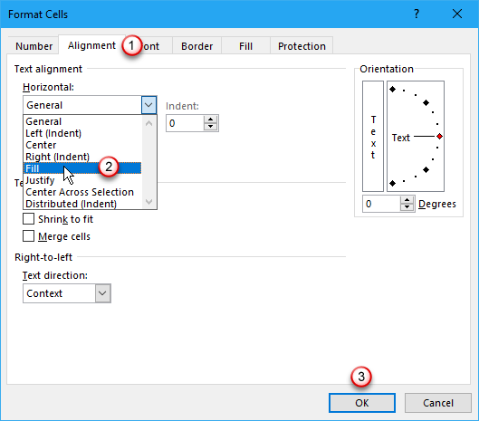
On the Format Cells dialog box, click the Alignment tab. Then, select Fill from the Horizontal dropdown list and click OK.
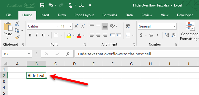
The overflow text in the first cell does not show even when there is nothing in the cell to the right.
How to Hide and Unhide Comments
Comments in Excel allow you to annotate your worksheets. This is useful when collaborating on worksheets. You can set reminders or add notes for yourself or for others or explain formulas or how to use part of a worksheet.
You may want to hide comments if there are many on your worksheet. The comments could make it hard to read your data.
By default, cells with comments contain a small red triangle in the upper-right corner called a comment indicator. These indicators can also be hidden.
To hide a comment on an individual cell, select the cell and do one of the following:
- Right-click the cell and select Show/Hide Comment.
- Click Show/Hide Comment in the Comments section of the Review tab.
To show the comment again, select the same cell and select or click Show/Hide Comment again.
You can also show or hide comments on multiple cells by using the Shift and Ctrl keys to select the cells and then select or click Show/Hide Comment.
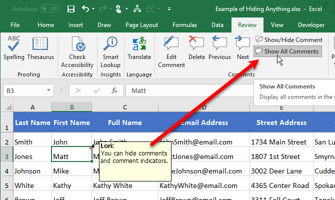
To show all comments at once, click Show All Comments in the Comments section on the Review tab. This option shows all the comments on all open workbooks. While this option is on, any workbooks you open or create will show all comments until you turn the option off.
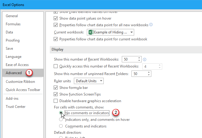
To hide both the comments and comment indicators, go to File > Options. Click Advanced on the left, then scroll down on the right to the Display section. Select No comments or indicators under For cells with comments, show. The indicators and comments are hidden, and the comments don’t display when you hover over cells.
To show the comments and indicators again, select one of the other two options under For cells with comments, show. You can also click Show All Comments in the Comments section of the Review tab.
The options under For cells with comments, show in the Excel Options and the Show All Comments option on the Review tab are linked. For more information about the behavior when hiding and showing comments, see our article about working with comments.
How to Hide and Unhide Certain Cells
You can’t hide cells themselves, but you can hide the contents of a cell. Maybe you have some data referenced by other cells that does not need to be seen.
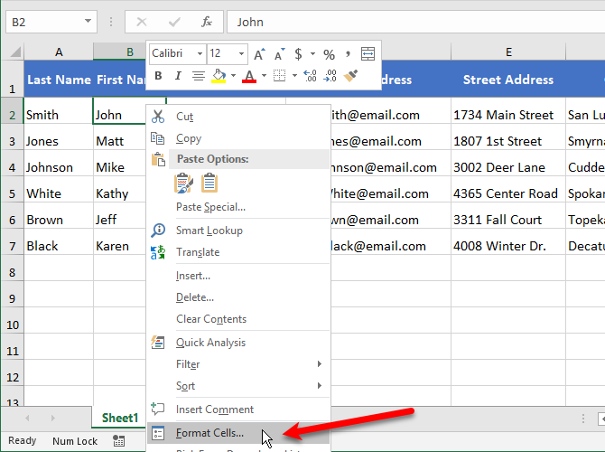
To hide the contents of a cell, select the cell(s) you want to hide (use Shift and Ctrl to select multiple cells). Then, do one of the following:
- Right-click on the selected cell(s) and select Format Cells.
- Press Ctrl + 1.
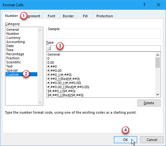
On the Format Cells dialog box, make sure the Number tab is active. Select Custom in the Category box.
Before changing the Type, note what’s currently selected. This way you know what to change it back to when you decide to show the content again.
Enter three semicolons (;;;) in the Type box and click OK.
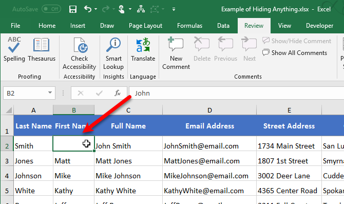
The contents in the selected cells is now hidden, but the value, formula, or function in each cell still displays in the Formula Bar.
The hidden content is still available to use in formulas and functions in other cells. If you replace the content in a hidden cell, the new content will also be hidden. The new content is available for use in other cells just like the original content.
To show the content in a cell again, follow the same steps above. But this time, choose the original Category and Type for the cell on the Format Cells dialog box.
How to Hide and Unhide the Formula Bar
When you hide a cell, as described in the previous section, you can still see the contents, formula, or function in the Formula Bar. To completely hide the contents of a cell, you must hide the Formula Bar also.
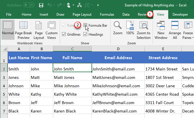
On the View tab, uncheck the Formula Bar box in the Show section.
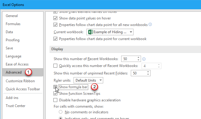
You can also hide the Formula Bar on the Excel Options dialog box.
Go to File > Options. Then, click Advanced on the left and uncheck the Show formula bar box in the Display section on the right.
How to Hide and Unhide Formulas
By default, when you enter a formula in a cell, the formula displays in the Formula Bar and the result displays in the cell.
If you don’t want others to see your formulas, you can hide them. One way is to hide the Formula Bar using the method in the previous section. But anyone can show the Formula Bar again.
You can securely hide a formula in a cell by applying the Hidden setting to the cell and then protecting the worksheet.
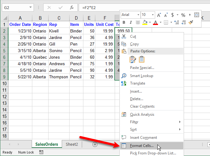
Select the cell(s) for which you want to hide the formula(s) and do one of the following:
- Right-click on the selected cell(s) and select Format Cells.
- Press Ctrl + 1.
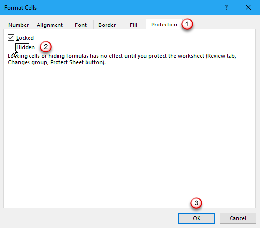
On the Protection tab, check the Hidden box. Then, click OK.
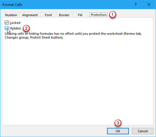
You still need to protect the sheet to hide the formulas.
Click Protect Sheet in the Protect section on the Review tab.
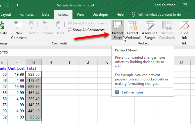
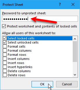
On the Protect Sheet dialog box, make sure the Protect worksheet and contents of locked cells box is checked.
In the Password to unprotect sheet box, enter a password to prevent others from unprotecting the worksheet. This is not required, but we recommend it.
By default, Select locked cells and Select unlocked cells are checked in the Allow all users of this worksheet to box. You can check boxes for other actions you want to allow users of your worksheet to perform, but you may not want to if you don’t want other users to change your worksheet.
Enter your password again on the Confirm Password dialog box.
The formulas in the selected cells do not show in the Formula Bar now. But you still see the results of the formulas in the cells, unless you’ve hidden the contents of those cells as described in the “How to Hide and Unhide Certain Cells” section above.
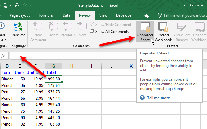
To show the formulas again, select the cells for which you want to show the formulas and click Unprotect Sheet in the Protect section of the Review tab.
If you entered a password when protecting the sheet, enter the password on the Unprotect Sheet dialog box that displays. If you didn’t protect the sheet with a password, no further prompts display.
The formulas won’t show just yet. You must turn off the Hidden setting for them.
Select the cells for which you hid the formulas and do one of the following:
- Right-click on the selected cell(s) and select Format Cells.
- Press Ctrl + 1.
Uncheck the Hidden box on the Protection tab and click OK.
The formulas for the selected cells will now be visible in the Formula Bar again if you haven’t hidden the Formula Bar.
How to Hide and Unhide Rows and Columns
If you want to remove one or more rows or columns from a worksheet, but you don’t want to delete them, you can hide them.
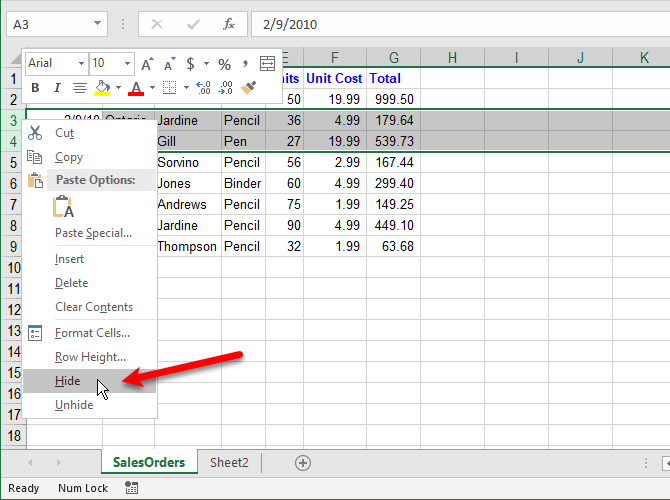
To hide one or more consecutive rows, first select the rows. Then, do one of the following:
- Right-click on the selected rows and select Hide.
- Press Ctrl + 9.
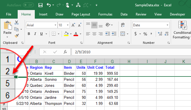
The selected rows are replaced with a double line in the row headings and a thick line where the rows were. When you click anywhere else on the worksheet, the thick line goes away. But you can tell where the hidden rows are by the missing row numbers and the double line in the row headings.
Cells in hidden rows and columns can still be used in calculations in other cells and can perform calculations on other cells while hidden.
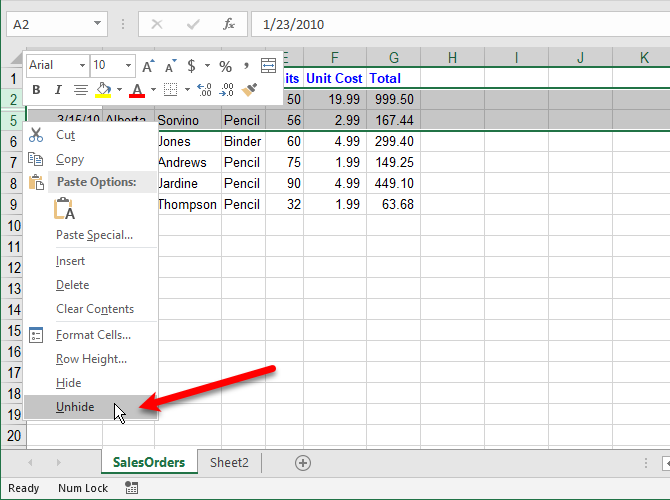
To unhide consecutive rows, select the rows above and below the hidden rows. Then, do one of the following:
- Right-click on the selected rows and select Unhide.
- Press Ctrl + Shift + 9.
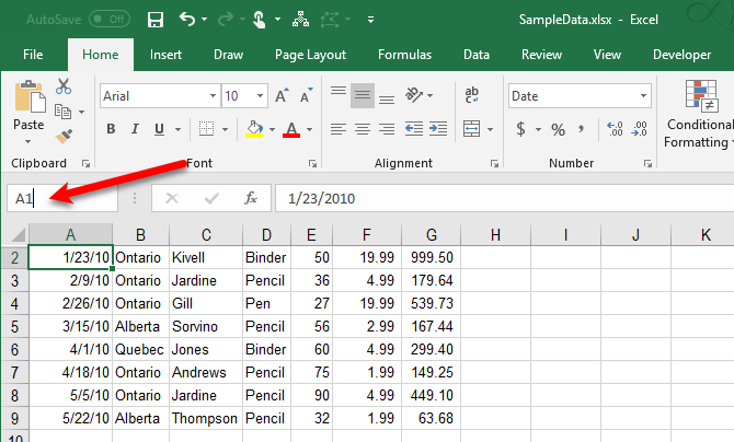
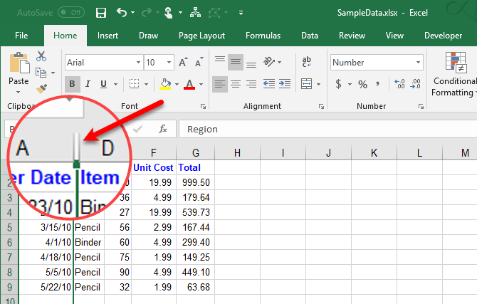
What if you hide the first row? This method of unhiding doesn’t work on the first row of a worksheet because there is no row above the first row.
To select the first row, click in the Name box to the left of the Formula Bar, type in “A1”, and press Enter. Then, press Ctrl + Shift + 9.
Hiding columns work like hiding rows. Select the column or consecutive columns you want to hide, and do one of the following:
- Right-click on the selected columns, and select Hide.
- Press Ctrl + 0 (zero).
The same double line and thick line you see when hiding rows display in place of the hidden columns. The column letters are also hidden.
To show the columns again, select the columns to the left and right of the hidden columns. Then, do one of the following:
- Right-click on the selected columns and select Unhide.
- Press Ctrl + Shift + 0 (zero).
If you’ve hidden the first column (A), you can unhide it like you do for when you hide the first row. To select the first column, click in the Name box to the left of the Formula Bar, type in “A1”, and press Enter. Then, press Ctrl + Shift + 0 (zero).
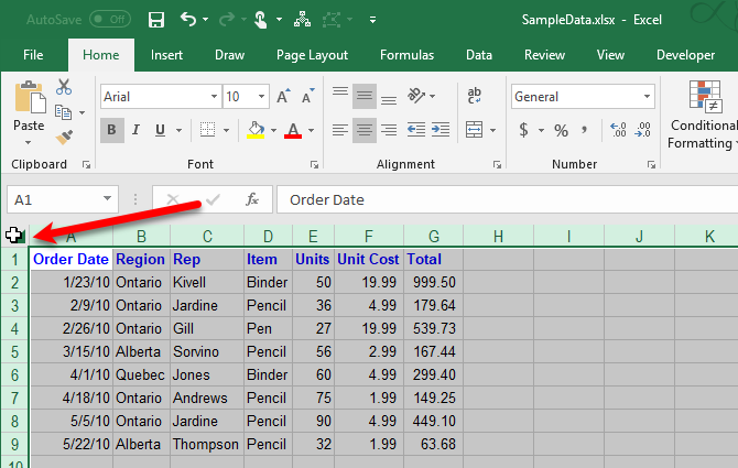
If you’ve hidden a lot of rows and columns, you can unhide all the hidden rows or columns at once.
Select the entire worksheet by clicking in the box between the row and column headers or pressing Ctrl + A. Then, press either Ctrl + Shift + 9 to unhide all the hidden rows or Ctrl + Shift + 0 (zero) to unhide all the hidden columns.
You can also right-click on the row or column headers while the entire worksheet is selected and select Unhide.
Show Only the Data You Want to Show in Excel
Hiding data is a simple but useful skill to learn in Excel, especially if you plan to use your worksheets in a presentation. Enter all the data you need, even if you only need some data for calculations or some is sensitive or private.
Read Full Article
No comments:
Post a Comment