How US national security agencies hold the internet hostage

Team Telecom, a shadowy US national security unit tasked with protecting America’s telecommunications systems, is delaying plans by Google, Facebook and other tech companies for the next generation of international fiber optic cables.

Team Telecom is comprised of representatives from the departments of Defense, Homeland Security, and Justice (including the FBI), who assess foreign investments in American telecom infrastructure, with a focus on cybersecurity and surveillance vulnerabilities.

Team Telecom works at a notoriously sluggish pace, taking over seven years to decide that letting China Mobile operate in the US would “raise substantial and serious national security and law enforcement risks,” for instance. And while Team Telecom is working, applications are stalled at the FCC.

The on-going delays to submarine cable projects, which can cost nearly half a billion dollars each, come with significant financial impacts. They also cede advantage to connectivity projects that have not attracted Team Telecom’s attention – such as the nascent internet satellite mega-constellations from SpaceX, OneWeb and Amazon.

Team Telecom’s investigations have long been a source of tension within Silicon Valley. Google’s subsidiary GU Holdings Inc has been building a network of international submarine fiber-optic cables for over a decade. Every cable that lands on US soil is subject to Team Telecom review, and each one has faced delays and restrictions.

Read Full Article

The FTC looks to change children’s privacy law following complaints about YouTube

The U.S. Federal Trade Commission is considering an update to the laws governing children’s privacy online, known as the COPPA Rule (or, the Children’s Online Privacy Protection Act). The Rule first went into effect in 2000 and was amended in 2013 to address changes in how children use mobile devices and social networking sites. Now, the FTC believes it may be due for more revisions. The organization is seeking input and comments on possible updates, some of which are specifically focused on how to address sites that aren’t necessarily aimed at children, but have large numbers of child users.

In other words, sites like YouTube.

The FTC’s announcement comes only weeks after U.S. consumer advocacy groups and Senator Ed Markey (D-Mass.) sent complaint letters to the FTC, urging the regulators to investigate YouTube for potential COPPA violations.

The advocacy groups allege that YouTube is hiding behind its terms of service which claim YouTube is “not intended for children under 13” — a statement that’s clearly no longer true. Today, the platform is filled with videos designed for viewing by kids. Google even offers a YouTube Kids app aimed at preschooler to tween-aged children, but it’s optional. Kids can freely browse YouTube’s website and often interact with the service via the YouTube TV app — a platform where YouTube Kids has a limited presence.

According to the letter written by the Campaign for a Commercial-Free Childhood (CCFC) and the Center for Digital Democracy (CDD), Google has now collected personal information from nearly 25 million children in the U.S., and it used this data to engage in “very sophisticated digital marketing techniques.”

The groups want YouTube to delete the children’s data, set up an age-gate on the site, and separate out any kids content into its own app where YouTube will have to properly follow COPPA guidelines.

These demands are among those pushing the FTC to this action.

The Commission says it wants input as to whether COPPA should be updated to better address websites and online services that are not traditionally aimed at children but are used by kids, as well as whether these “general audience platforms” should have to identity and police the child-directed content that’s uploaded by third parties.

In other words, should the FTC amend COPPA so it can protect the privacy of the kids using YouTube?

“In light of rapid technological changes that impact the online children’s marketplace, we must ensure COPPA remains effective,” said FTC Chairman Joe Simons, in a published statement. “We’re committed to strong COPPA enforcement, as well as industry outreach and a COPPA business hotline to foster a high level of COPPA compliance. But we also need to regularly revisit and, if warranted, update the Rule,” he added.

While YouTube is a key focus, the FTC will also seek comment on whether there should be an exception for parental consent for the use of educational technology in schools. And it wants to better understand the implications for COPPA in terms of interactive media, like interactive TV (think Netflix’s Minecraft: Story Mode, for example), or interactive gaming.

More broadly, the FTC wants to know how COPPA has impacted the availability of sites and services aimed at children, it says.

The decision to initiate a review of COPPA was a unanimous decision from the FTC’s five commissioners, which includes three Republicans and two Democrats.

Led by Simons, the FTC in February took action against Musical.ly (now TikTok), by issuing a record $5.7 million fine for its COPPA violations. Similar to YouTube, the app was used by a number of under-13 kids without parental consent. The company knew this was the case, but continued to collect the kids’ personal information, regardless.

“This record penalty should be a reminder to all online services and websites that target children: We take enforcement of COPPA very seriously, and we will not tolerate companies that flagrantly ignore the law,” Simons had said at the time.

The settlement with TikTok required the company to delete children’s videos and data and restrict underage users from being able to film videos.

It’s unclear why the FTC can’t now require the same of YouTube, given the similarities between the two services, without amending the law.

“They absolutely can and should fine YouTube, not to mention force YouTube to make significant changes, under the current regulations,” says Josh Golin, the Executive Director for CCFC. “As for the YouTube decision – by far the most important COPPA case in the agency’s history – it’s extremely concerning that the Commission appears to be signaling they do not have the authority under the current rules to hold YouTube accountable,” he says.

“COPPA rules could use some updating but the biggest problem with the law is the FTC’s lack of enforcement, which is something the Commission could address right away without a lengthy comment period,” Golin adds.

The FTC says it will hold a public workshop on October 7, 2019 to examine the COPPA Rule.

Read Full Article

Google creates massive-scale tribute to Apollo 11 software lead Margaret Hamilton

Google has a number of different celebrations of the 50-year anniversary of the Apollo 11 Moon landing going on right now, but one organized by the Maps team might be the most grandiose in terms of scale and effect. At the Ivanpah Solar Facility in the Mojave Desert, Google set about creating a huge portrait celebrating Apollo program lead software engineer Margaret Hamilton, using reflective solar panels and the light of the Moon.

The portrait is made up of over 107,000 mirrors, which cover an area spanning 1.4-square miles, which is actually bigger in surface area than Central Park in NYC – or, for a different sense of scale, it’s an area that would fit over 200 Eiffel Towers lined up side-by-side. You could spot the image created from as high up as 1,900 meters (about 6,233 feet).

[gallery ids="1857488,1857490,1857489,1857491,1857487"]

The gigantic image includes not only a portrait of Hamilton, but also her name along with the ‘Apollo 11’ mission title, and an image of the lunar lander used to bring astronauts to the surface for the first time. That’s in reference to Hamilton’s key role in ensuring that the Apollo 11 landing went as planned, thanks to her creation of a priority display that provided astronauts with the info they needed despite an overloaded guidance computer near the end of the lander’s trip to the surface.

Hamilton, now 82, recently provided an interview to The Guardian detailing her path to Apollo and her role leading the software team for the Apollo 11 mission.

Read Full Article

Google will now pay bigger rewards for discovering Chrome security bugs

Bug hunting can be a lucrative gig. Depending on the company, a serious bug reported through the proper channels can earn whoever found it first tens of thousands of dollars.

Google launched a bug bounty program for Chrome in 2010. Today they’re increasing the maximum rewards for that program by 2-3x.

Rewards in Chrome’s bug bounty program vary considerably based on how severe a bug is and how detailed your report is — a “baseline” report with fewer details will generally earn less than a “high-quality” report that does things like explain how a bug might be exploited, why it’s happening, and how it might be fixed. You can read about how Google rates reports right here.

But in both cases, the potential reward size is being increased. The maximum payout for a baseline report is increasing from $5,000 to $15,000, while the maximum payout for a high quality report is being bumped from $15,000 to $30,000.

There’s one type of exploit that Google is particularly interested in: those that compromise a Chromebook or Chromebox device running in guest mode, and that aren’t fixed with a quick reboot. Google first offered a $50,000 reward for this type of bug, increasing it to $100,000 in 2016 after no one had managed to claim it. Today they’re bumping it to $150,000.

They’ve also introduced a new exploit category for Chrome OS rewards: lockscreen bypasses. If you can get around the lockscreen (by pulling information out of a locked user session, for example,) Google will pay out up to $15,000.

Google pays additional rewards for any bugs found using its “Chrome Fuzzer Program” —a program that lets researchers write automated tests and run them on lots and lots of machines in the hopes of finding a bug that only shows up at much larger scales. The bonus for bugs found through the Fuzzer program will be increased from $500 to $1000 (on top of whatever reward you’d normally get for a bug in that category.)

Google says that it’s paid out over $5M in bug bounties through its Chrome Vulnerability Rewards Program since it was introduced in 2010. As of February of this year, the company had paid out over $15M across all of their bug bounty programs.

Read Full Article

Google teams up with Apollo 11 astronaut to celebrate the 50th anniversary of the Moon landing

It’s the 50th anniversary of the Moon landing, so it’s no surprise that Google’s daily doodle celebrates this milestone today. To mark the event, Google teamed up with NASA and Michael Collins, the astronaut who piloted the command module while Neil Armstrong and Buzz Aldrin descended to the Moon.

Besides the usual doodle and animation, Google’s team created a video with Collins in which he narrates the sequence of events from his perspective. Not a lot of people can say that they orbited the Moon while sipping on a hot cup of coffee, after all.

It’s a fun video to watch, maybe precisely because it features Collins, who most people probably don’t know all that much about.

Earlier this month, Google also launched a couple of other Apollo 11-themed experiences, including an AR recreation of the command module that you can see after you search for “Apollo 11” on your Android or iOS phone.

Read Full Article

Facebook accused of contradicting itself on claims about platform policy violations

Prepare your best * unsurprised face *: Facebook is being accused of contradicting itself in separate testimonies made on both sides of the Atlantic.

The chair of a UK parliamentary committee which spent the lion’s share of last year investigating online disinformation, going on to grill multiple Facebook execs as part of an enquiry that coincided with a global spotlight being cast on Facebook as a result of the Cambridge Analytica data misuse scandal, has penned another letter to the company — this time asking which versions of claims it has made regarding policy-violating access to data by third party apps on its platform are actually true.

In the letter, which is addressed to Facebook global spin chief and former UK deputy prime minister Nick Clegg, Damian Collins cites paragraph 43 of the Washington DC Attorney General’s complaint against the company — which asserts that the company “knew of other third party applications [i.e. in addition to the quiz app used to siphon data off to Cambridge Analytica] that similarly violated its Platform Policy through selling or improperly using consumer data”, and also failed to take “reasonable measures” to enforce its policy.

The Washington, D.C. Attorney General, Karl Racine, is suing Facebook for failing to protect user data — per allegations filed last December.

Collins’ letter notes Facebook’s denial of the allegations in paragraph 43 — before raising apparently contradictory evidence the company gave the committee last year on multiple occasions, such as the testimony of its CTO Mike Schroepfer, who confirmed it is reviewing whether Palantir improperly used Facebook data, among “lots” of other apps of concern; and testimony by Facebook’s Richard Allen to an international grand committee last November when the VP of EMEA public policy claimed the company has “taken action against a number of applications that failed to meet our policies”.

The letter also cites evidence contained in documents the DCMS committee seized from Six4Three, pertaining to a separate lawsuit against Facebook, which Collins asserts demonstrate “the lax treatment of abusive apps and their developments by Facebook”.

He also writes that these documents show Facebook had special agreements with a number of app developers — that allowed some preinstalled apps to “circumvent users’ privacy settings or platform settings, and to access friends’ information”, as well as noting that Facebook whitelisted some 5,200 apps “according to our evidence”.

“The evidence provided by representatives of Facebook to this Select committee and the International Grand Committee as well as the Six4Three files directly contradict with Facebook’s answer to Paragraph 43 of the complaint filed against Facebook by the Washington, D.C. Attorney General,” he writes.

“If the version of events presented in the answer to the lawsuit is correct, this means the evidence given to this Committee and the International Grand Committee was inaccurate.”

Collins goes on to ask Facebook to “confirm the truthfulness” of the evidence given by its reps last year, and to provide the list of applications removed from its platform in response to policy violations — which, in November, Allan promised to provide the committee with but has so far failed to do so.

We’ve also reached out to Facebook to ask which of the versions of events it’s claimed are true is the one it’s standing by at this time.

Read Full Article

Who Unfollowed Me on Instagram? Here’s How to Find Out

How to Avoid Fake Ads Disguised as Fake Download Links

While ads are a necessary part of the internet, not all advertisements are created equal. One of the most common kinds of fake ads are “download” buttons that don’t lead to the software you were looking for.

These ads masquerading as download buttons are a huge pain. Let’s look at why they exist, how to spot them, and how to avoid the ads.

Why Do Fake Download Button Ads Exist?

You might wonder where these fake download ads come from in the first place. They almost never lead to anything helpful—instead, they bring you to malware, junky software, or phishing sites. So why are they so prevalent?

The answer, unfortunately, is that their deception works. It’s difficult to get users to click on ads most of the time, since most people have become better at recognizing them. But when you’re already looking for a download link or button, you’re more likely to fall for a fake one.

Additionally, someone falling for these is a good indicator that they’ll be prone to future scams.

Why These Ads Keep Appearing

So we know why scammers love these ads, but why do websites allow them? In many cases, it’s because they can’t get many other advertisers. Reputable companies aren’t exactly jumping to show their ads on sites like torrent trackers and file-sharing services, especially because they’re often associated with illegal activity.

These websites have to pay their bills somehow, so they go with these ads and apparently don’t mind the implications to less tech-savvy users.

Despite all this, you’ll still occasionally see fake download ads appear on mainstream sites like MakeUseOf. We don’t want or allow them, but they show up anyway. Though most of our ads come from Google, we don’t have the ability to approve what ads appear on the site ahead of time.

Bad actors constantly play whack-a-mole with Google and webmasters, trying to get their fake ads through the system. Websites report the ads when they appear; Google blocks these companies from creating more ads, but new ones still pop up all the time.

How to Spot Fake Download Ads

As long as these ads keep getting through the system, you should know what one looks like when you see it. This will keep you safe and make sure you only use actual download links.

As a general rule, most legitimate sites do not use giant Download buttons. You’ll usually find the real download link as a link in text form, such as the download links at the bottom of sections in MakeUseOf articles. However, many dedicated software download sites do use a similar green button for downloads, making it harder to tell.

A huge giveaway that you’re looking at a fake download button is the AdChoices logo in the top-right corner. This is a regulatory program that many advertisers are part of, which calls for certain principles in ads.

If you see this icon, it’s quite likely a Google ad, meaning it’s not a real download. When you spot one, you should click the X icon. This allows you to report the ad and lets the service know you don’t want to see it again.

In addition, ads are sometimes marked clearly with Advertisement next to them, which is another telltale sign.

Testing the URL

Another way to tell if a download link is genuine is by hovering over it. Every major browser will show you a little tooltip with the destination URL of the link. If you see googleads or something similar at the start, it is not a valid download link. Typically, genuine links are relatively short and have the software’s name in them.

If you’re really not sure, you can use a web service to see if the link is safe, then click the button to test it if it seems safe to proceed. Pay attention to what happens next—does it start a file download? If so, look at the file name and extension.

Windows software is most often packaged as an EXE or ZIP file. Mac programs are usually in DMG or ZIP format (though you can find a good bit of Mac software on the safe App Store). In both cases, the downloaded installer should have the name of the program you’re looking for. Files with generic names like AppDownloader.exe will typically bundle in extra garbage.

Should you see a load of additional ads or a completely unrelated website when you click a button, get out. That’s not the site you’re looking for. And if you’re really not sure whether the file you downloaded is trustworthy, scan it with your antivirus. You may also want to get a second opinion using Malwarebytes or a web scanner like VirusTotal.

Download From Safe Sites Instead

Now you should know how to identify fake downloads when you see them. This will come in handy when using filesharing sites, where you often don’t have another option for downloading what you’re after.

But in many cases, it’s possible to bypass the above concerns and avoid ads meant to trick you. You simply need to download from a reputable service.

If you’re looking to install a well-known program, one of the best places to do so is through the official website. This is much less likely to have fake download buttons (and any bundled junk) than random redistributors. Simply Googling “download [app]” will provide a box linking to the official page in many cases.

Otherwise, take a look at our list of the safest sites for installing Windows software. These will let you grab popular apps without having to worry about clicking on fake ads. Likewise, make sure you stay away from dangerous software download services.

Avoiding Fake Downloads Is Crucial

As long as these fake ads remain profitable for scammers, we’ll probably never see the end of them. In most cases, you should avoid download from sites with loads of fake ads if you can, because they’re probably not trustworthy. Whether by using a more reliable site or cutting through the deception, these tips will help you dodge the fakes.

Counterfeit download buttons aren’t the only shams to watch out for online. See our guide to spotting other online fakes so you’re prepared for anything.

Read the full article: How to Avoid Fake Ads Disguised as Fake Download Links

Read Full Article

The 10 Best Podcasts for Kids to Keep Them Entertained

Podcasts are the perfect way to learn new things, hear interesting stories, or just have a laugh. You’ve probably listened to at least one by now, but have your kids listened to any podcasts? To help them get started, these are the best podcasts for kids.

There are a wealth of interesting podcasts for kids available, and we’ve rounded up some of the best. These podcasts can entertain curious minds, and are perfect to fire children’s imaginations. Here are the best podcasts for kids.

1. Circle Round

Circle Round is a storytelling podcast aimed at children aged between four and 10. It takes traditional folk tales and updates them for a modern, diverse audience. It represents all cultures and aims to teach children values like kindness and persistence.

Some of the audio plays feature famous voices and every episode features original music. Plus, the stories end with a question, aimed to spark a discussion amongst family and friends.

2. Brains On!

Brains On! is a fun weekly science podcast that covers all sorts of topics. Your kids will learn how animals see the world, how sound waves work, why humans smell, and so much more. Chances are, any adult listening along will learn a thing or two as well.

Children can send in their worldly ponders to be answered. Regular host Molly Bloom is on hand to help answer questions, joined by a different kid every episode. This is the perfect podcast for curious children.

3. Ear Snacks

Teeth, cracks, puzzles… anything and everything is covered in Ear Snacks. The two hosts, Andrew Barkan and Polly Hall, spend each episode exploring a topic alongside a number of parents, kids, and experts.

The unique element is that this a musical podcast. There’ll be random bursts of original songs that are not only catchy, but educational too. It won’t be long before your kids are singing all about grapes or the body parts of a bug.

4. What If World

Kids love inventing things and asking questions, so What If World is the perfect combination. Every episode opens with a theoretical (often silly) question from a listener. What if cats ruled the world? What if rich ghosts were bad at selling cars? Or even, what if french fries and drinks went to war?

Host Eric O’Keeffe tackles all of these wacky questions and turns them into fun, engaging stories that also include life lessons. Not only will your children have their imaginations sparked, but they’ll also accidentally learn good morals along the way.

5. The Unexplainable Disappearance of Mars Patel

Mars Patel is a scripted serial mystery, described by its creators as Goonies meets Spy Kids meets Stranger Things for middle grade kids. It has great writing and sound design and will be sure to grip children with its exciting twists and turns.

One of the great things about this podcast, which currently has three seasons, is that the cast consists of kids. They all act really well and it lends authenticity to the story. Good luck tearing your young ones away from this podcast.

6. Pants on Fire

Pants on Fire is a game show perfect for the era of fake news and how quickly it spreads. Each week, a kid interviews two adult experts about all sorts of topics, like detectives, magic, and puppets.

But here’s the twist: one of those experts is a big liar. They’re making all of their answers up. It’s pacy, quick-witted, and packed full of sound effects. The show encourages children to ask insightful questions, analyze what is presented to them, and know how to make informed decisions.

7. Chompers

Chompers is a twice-daily podcast that is meant to be played when your kids are brushing their teeth, targeted at youngsters aged between three and seven. Episodes may feature jokes, stories, fun facts, songs, interviews, and so much more.

Dentists recommend brushing your teeth for at least two minutes, and so Chompers is designed to run that perfect bite-sized length of time. Alongside the fun content, it also lightly guides your kids through their brushing—ensuring they remain entertained and sparkling.

8. Good Night Stories for Rebel Girls

Good Night Stories for Rebel Girls is a bestselling book series that has been turned into a podcast. It aims to encourage the next generation by telling stories about extraordinary women.

Carmen Amaya, Celia Cruz, and Mary Kom are just a few of the women across the world, from the past and present, that this podcast covers. If you want an inspirational listen for your kid, this is the one.

9. Smash Boom Best

Every episode of Smash Boom Best takes two topics and pits them against one another, letting the children decide which they think is victorious. Things up for debate include invisibility versus flying, unicorns versus dragons, and chocolate versus cheese. All important topics, we’re sure you’ll agree.

The debaters must use facts, persuasion, and their passion to try to win their case. Just a word of warning: your kids might start challenging you to debate after listening to this one!

10. Book Club for Kids

Podcasts are all about listening, of course, but they can also be about reading. Book Club for Kids is a 20-minute podcast hosted by Kitty Felde, which sees a small group of middle grade students discussing their favorite books.

Episodes also include celebrity readings and interviews with authors. The books covered include some famous ones, like the Harry Potter and Divergent series, but also lesser known recommendations too. Any young, voracious readers will love Book Club for Kids.

The Best Podcasts for Kids

Hopefully you’ve found a podcast or two here that is perfect for your kids. It’s a great way to get them away from their screen and help them learn things, even if they don’t realize it. And the chances are they’ll soon find their own favorite podcasts to listen to.

If your child is older and owns a smartphone, you might want to let them use a podcast app to consume these audible delights. If so, check out our look at the most popular podcast apps, compared.

And if you want even more podcast recommendations then take a look at our list of family-friendly podcasts you can listen to with your kids.

Image Credit: welcomia/Depositphotos

Read the full article: The 10 Best Podcasts for Kids to Keep Them Entertained

Read Full Article

Android Phone Speakers Not Working? Here Are 7 Fixes to Try

How to Use the Name Box in Excel

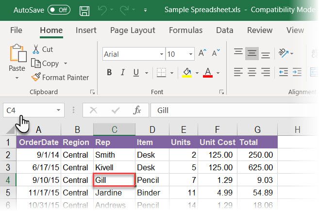
You can’t go anywhere in Microsoft Excel without using this humble little box. But where is the Name Box in Excel? It lies right next to the formula bar in a worksheet and displays the address of the selected cell or an object. But that’s just the most obvious use. You can navigate around the sheet with it or use it as a powerful selection tool.

But that’s just the scratching the corners of the box. Let’s look at all the productivity purposes the Name Box was created for.

1. Find the Address of the Selected Cell

As shown in the screen above, the Name Box shows C4 because the cell C4 is selected right now. Click on any cell to get the cell address to use in a formula.

The Name box won’t just give you the address of one cell. It can be applied to any group of cells too. For instance:

Select a block of cells. The Name Box will identify the first cell in the selected group of cells.

Select a range of non-contiguous cells. You can select several cells that are not grouped together. Press the Ctrl key and choose a bunch of non-contiguous cells. The Name Box in Excel will display the address of the last cell you select.

You can go the other way also. If you want to go to a specific cell or a range of cells, then you can type the address of that cell in this Name Box and select them in a pinch.

Let’s see how it can speed up your work when you have a lot of rows, columns, and even sheets to work with.

2. Use the Name Box to Select Cells

Let’s do away with the mouse to select a block of cells with their addresses alone.

Select a block of cells. In the screenshot below, I typed A2:B10 in the Name Box and then pressed Enter. This selects a block of cells and you didn’t have to travel across your worksheet with the mouse.

Select a range of cells on another worksheet. Add the sheet reference (E.g. Sheet2!A5:B10) in the Name Box.

Select multiple blocks of cells. As shown with an example in the screen below, you can type A1:A5,C1:C5,G1:G5 and then press Enter to select any number of non-adjacent blocks of cells at once.

You can jump from any cell to any cell by just typing these cell addresses. To jump to any cell in another worksheet within the same workbook, type the sheet name, an exclamation point, the cell address, and then press Enter. For example, Sheet2!A10.

3. Select Rows and Columns With the Name Box

Use the Excel Name Box as another speed trick to quickly select rows and columns. These are handy Excel shortcuts when you want to want to avoid the mouse.

Select the current row. Type the letter R in the Name Box and press Enter to select the current row.

Select the current column. Type the letter C in the Name Box and press Enter to select the current column.

Do remember that the letters R and C are reserved by Excel for this reason, and you cannot use these single alphabets to create Named Ranges in Excel (learn more about Named Ranges below).

Select any number of rows. Want to highlight the first five rows? Type 1:5 in the Name Box and then press Enter to select rows 1 through 5. You must select two or more rows. If you type a single number in the Name Box (for instance, 1) and press Enter, Excel shows an error message.

Select two or more columns. Want to highlight the first five columns? Type A:E in the Name Box and then press Enter to select columns A through E. Again, you have to give two or more columns.

Select Specific Rows and Columns Together. You can even select several multiple rows and columns together. For instance, type A:C,5:7 and hit Enter to get the following selection.

This is interesting because you can immediately see where rows and column values overlap. In the screen below, it is the data in the range A5:C7.

In the above case, you can also just isolate the overlap between cells by typing A:C 5:7. Omit the comma and include a single space between the ranges to see that Excel highlights the cells where the two ranges intersect.

Find the total number of rows and columns. The Name Box displays the total number of rows and columns when you keep the left mouse button pressed or hold down the Shift key while selecting a block of cells.

4. Create Named Ranges for Excel Formulas

Imagine an Excel worksheet that references several cell ranges in multiple formulas. It’s easy to get confused with all the alpha-numeric cell names. Wouldn’t it be easier if these cells had their own descriptive names that told you at a glance what the cells were all about?

Excel uses Named Ranges to do just that. And you will use the Name Box in Excel for that.

1. Select a cell or a range of cells.
2. Give a descriptive name to the selection in the Name Box. Press Enter.
3. Use this name instead of selected cell address or the address of the entire range in any formulas.

In the screen below, I assigned the name Interest to cells B3 to B7. I select the range of these cells, typed the word Interest in the Name Box, and then hit Enter. All range names in a workbook must begin with a letter, underscore, or backslash. Spaces are not allowed.

See this illustrated step by step tutorial to learn how to work with Named Ranges in Excel. Named Ranges are excellent descriptors if you also program with macros in Excel.

5. Name Every Object in Your Excel Worksheet

A worksheet can have different objects like pictures, charts, macro buttons, form controls like buttons and checkboxes, etc. Excel uses generic names like Chart 1, Chart 2… to name them. You can navigate through all objects by typing these names in the Name Box.

But just like the facility of Defined Ranges for easier formulas, you can assign objects your own descriptive names. It makes them easier to find.

1. Select the chart, picture, or object.
2. Place the cursor in the Name Box and type a new descriptive name.
3. Press Enter.

6. Insert (Or Delete) Multiple Blank Rows With the Name Box

There are several ways to insert blank rows in Excel. One of them is with the Name Box. This method is useful when you want to insert many rows in one shot. Head to the Name Box and use the format starting row: ending row with the numeric values for the rows you want.

For example, if you want to insert 10 rows from row 2, then type 2:11 in the Name Box and hit Enter. Excel will select the next ten rows starting from row 2 (it is “eleven” because the second row will also be counted in the next ten row) selections.

Then, right click on the selected rows and click Insert. Ten blank rows will be inserted starting from row 2.

This method is handy when you want to insert thousands of blank rows for some reason.

7. View a Macro

As mentioned before, you can give your own names to macro buttons in Excel. But you can also launch the Visual Basic editor to get into the source code for any macro.

Type the name of the macro in the Name Box. The VBA Editor opens with the macro’s source code for you to edit or see.

The Name Box in Excel Is a Productivity Shortcut

The time saving uses of Excel’s Name Box demonstrate why you shouldn’t neglect it’s utility. As it is a core navigational feature in Excel, you just have to use it. But creating Named Ranges and its prowess for quick selections show how you can better grasp a complex spreadsheet.

That’s just the start you need to use more of Excel’s time saving secrets to boost your productivity.

Image Credit: Rawpixel/Depositphotos

Read the full article: How to Use the Name Box in Excel

Read Full Article

How to Find the Best Discord Servers

Discord started out as a voice chat program for gamers. But it has since grown to become a popular location for hosting text-based forums as well. There are specific Discord servers for all sorts of interests, including games, movies, music, and more.

However, it’s not always easy to find servers to join. If you’re new to Discord, you might be wondering where to start. Here are all the best ways you can find the best Discord servers that match your interests.

1. Find Servers Using the Discord Server Directory

Whether you’re using the Discord webapp or the Discord app on your phone, look in the far-left column. Under the icons for the servers you are currently a member of, there is a round magnifying glass icon. Click on this and you’ll be taken to the official Discord server directory.

The homepage of the directory shows you some of the most popular servers, like the Official Fortnite server or the Official Minecraft server. These servers have hundreds of thousands of members and are among the largest on Discord.

If you want to check out a server, hover over its name and you’ll see a blue button that says View. Click this to be taken to the server, which you can look through before deciding if you want to join. If you like what you see, you can join the server by clicking Join Server at the bottom of the screen. Or click Back to Discovery to be taken back to the server directory.

You can also use the search bar in the directory to search for servers dedicated to particular topics. Or you can use the drop-down menu to search for servers in a particular language.

Download: Discord for Android | iOS

2. Find Discord Servers Using the Disboard Website

Another way to find the best Discord servers is to use the Disboard website. Disboard has a list of Discord servers for all types of topics, including many gaming communities and anime and manga fanbases. It also lists servers for topics like music, technology, movies, memes, and roleplay.

To find a server, you can browse the Disboard directory using the Categories and Popular Tags on the main page. Categories are listed in pale blue, and popular tags are listed in green. Click on a topic to bring up a list of Discord servers related to that topic.

Once you click a topic, you’ll see more information about each listed server, like its name, a starred user review rating, a description of the server, and how many people are currently online. You’ll also see a flag to indicate the language of the server and an icon at the bottom if it is a server which allows NSFW content.

Alternatively, you can add a term to the search bar to search for servers related to that topic. Or, for more personal recommendations, click on Reviews at the top to see user reviews of different servers.

When you find a server you like the look of, click the Join this server button at the bottom of the posting and you’ll be taken to an invite page from which you can enter the server.

3. Find Servers Using the DiscordMe Website

Another website which offers a list of Discord servers is Discord.me. This site leans slightly more towards listing anime servers, but there are plenty of listings for gaming, entertainment, and social categories as well.

To find a server, you can browse the most popular servers from the home page. Or use the Categories drop-down menu at the top of the page to search for a server by category, like anime, crypto, eSports, education, or gaming. Click on a category name to be taken to a list of the top servers in that category.

There’s also a fun Random feature in the left hand menu, accessed by clicking on the three horizontal lines in the top-left. This will take you to information about a random server from the directory.

You’ll see some servers listed as Platinum or Gold with a banner in the top-left. But don’t worry, as a user you do not have to pay to access any server. The platinum or gold designations indicate the server owner has paid to promote their server on Discord.me but you can still access it for free.

Once you have clicked on a server name you’ll see information about its categories, information about the server, and a banner image. Click on Join Server to be taken to the Discord invite page from which you can access the server.

4. Find Discord Servers From Your Favorite Websites

Another option for finding servers is to look for servers run by your favorite websites or tech influencers.

For example, popular technology forum Linus Tech Tips has its own Discord Server with information about hardware, gaming, and more. Other sites have exclusive Discord servers for particular groups of fans, such as Patreon supporters.

Many Twitch streamers have their own Discord servers as well, which can be a fun way to meet other people who are into the same games as you. Have a look around sites you visit regularly to see if they mention a Discord server.

5. How to Find Private Discord Servers

As well as public servers, there are also private Discord servers which require an invitation for you to join. You can often find invites to private servers on other social media sites like Twitter, Facebook, or Steam.

These servers typically have between 50 and 500 users, so they’re much smaller than the big public servers. That means they’re less active, but they can also have a better sense of community. If you find big servers to be impersonal or filled with drama, then a smaller private server might be more to your tastes.

If you’re looking for gaming servers, then Reddit is a good place to search. You’ll find a link like https://ift.tt/2XQf7mh which you can click and you’ll be taken to a landing page. Click on Accept Invite to be taken to the server.

Once you arrive in a server, check out the rules and guidelines. Some private servers will require you to message a mod or confirm you have read the rules before you’re given access to the rest of the channels.

Find the Best Discord Servers for Your Interests

There are Discord servers out there for almost any interest you can think of, and you can use these methods to find one that suits you.

If you’re a gamer using Discord, you might also want to check out Discord’s Steam-style game store which hosts a variety of games for you to play.

Read the full article: How to Find the Best Discord Servers

Read Full Article

The Humbird Can Turn Any Hollow Surface Into a Speaker

There aren’t a lot of advancements made in the world of speakers. Yes, they become more powerful and smaller, but the core design of a speaker hasn’t changed all that much in recent years.

However, one exception to that comes from bone conduction technology, which is designed to use vibrations on hollow surfaces to create sound. A cool new speaker called Humbird promises to be the smallest bone conduction speaker on the market, and we have to say, it sounds quite promising.

What Makes Humbird Special?

One thing that really makes Humbird stand out from the crowd is how small it is. It weighs in at just 35g and is only 1.57-inches in diameter. The creators claim it’s the smallest speaker of this type on the market right now, which is quite impressive.

The speaker uses Bluetooth to connect to just about any device, and if you have two Humbirds, you can sync them up for wireless stereo sound.

The creators promise that setting their speaker on different surfaces will create different types of sounds, so if you’re looking for something with some extra bass or cleaner highs, you can probably find a place to put Humbird to get the sound you’re after.

Some examples cited on the products Kickstarter page include a wooden desk for heavy voice and volume that doesn’t get too loud, a drum for thumping bass, an empty cardboard box for loud sound, and so on. Basically, as long as the surface upon which you set the speaker isn’t too thick, you’ll be able to get some kind of sound out of it. You’ll need to experiment to see what surfaces work well for you.

Obviously, one of the key things to know about a speaker like this is how loud it’ll go. According to the creators, you can actually reach volumes of up 115db, though it’ll depend on the surface.

When Is the Humbird Available?

Duramobi, the company behind Humbird, is currently seeking funding for its device on Kickstarter. It’s already exceeded its goal, so the device should find its way to market. If you’re interested in pre-ordering one, you can do so for HK$186 ($24 USD). If you want to get a pair of speakers to take advantage of the stereo functionality, you can snag a pair for HK$312 ($40 USD).

The company plans to ship the first batch of speakers to backers in August 2019, but as is always the case with crowdfunding campaigns, there are risks involved and there’s no guarantee that things come to fruition.

Read the full article: The Humbird Can Turn Any Hollow Surface Into a Speaker

Read Full Article

4 Courses Every Aspiring Entrepreneur Needs to Take

You don’t need a college degree to start a business. But to be successful, it’s essential to have some key skills under your belt. You can spend thousands on online courses, but there is a smarter way. From knowing where to invest your money in analyzing your sales, these courses should put you on the right path — now with up to 97% off at MakeUseOf Deals.

“Wall Street Training” Course Bundle

To be a successful entrepreneur, you need to understand finance and how to invest your money wisely. This training bundle shows you how, with 15 hours of video lessons. Along the way, you learn how to calculate risk, forecast your profits and compare financial statements. Worth $650 in total, the bundle is now just $89.

The Ultimate Data & Analytics Bundle: Lifetime Subscription

Using data is essential if you want to compete in business today. This huge course bundle offers 1,500 hours of certificated training on big data, covering SAS, R, Oracle, and more. In addition, you learn about data science, machine learning, analytics, and visualization. Order now for $29 to get lifetime access to all the courses, worth $299.

Evan Kimbrell’s Business Launching Bundle

Evan Kimbrell is the inspirational founder of Sprintkick, an agency that has developed over 100 apps. Nowadays, he’s one of the most popular instructors on Udemy. This bundle brings together 108 hours of his wisdom, from ideation to outsourcing and app development. You can get it now for $39, saving over $1,150.

The Ultimate AWS Data Master Class Bundle

Most digital startups are based in the cloud nowadays. This bundle of courses helps you master Amazon Web Services, one of the most popular cloud platforms. The nine courses also cover in-demand data skills, including DevOps and Kubernetes. Worth $1,679, the training is now only $39 with this bundle.

Like this deal? Check out Vault — you’ll get four premium tools, including NordVPN and Dashlane, to supercharge your online security. Try it free for 14 days now!

Prices are subject to change.

Read the full article: 4 Courses Every Aspiring Entrepreneur Needs to Take

Read Full Article

Watch an unfiltered interview of PicsArt founder at Disrupt Berlin

Smartphones have become a creative playground thanks to cameras and innovative apps, such as PicsArt. With PicsArt, anybody can add filters, stickers and tweak photos and videos in many different ways. It has been a massive hit with 130 million monthly active users. And that’s why I’m excited to announce that PicsArt founder and CEO Hovhannes Avoyan is joining us at TechCrunch Disrupt Berlin.

PicsArt started with a simple app that lets you edit photos before sharing them. There are many companies in this space, including VSCO, Snapseed and Prisma. But PicsArt has managed to become a cultural phenomenon in many countries including China.

If you’re thinking about editing a photo or video in one way or another, chances are you can do it in PicsArt. In addition to traditional editing tools (cropping, rotating, curves, etc.), you can add filters, auto-beautify your face, change your hair color, add stickers and text, cut out your face and use masks just like in Photoshop… I’m not going to list everything you can do because it’s a long list.

The result is an app packed with features that lets you express yourself, create visual storytelling and improve your social media skills. If you’re an Instagram user, chances you’ve seen more than one photo that has been edited using PicsArt.

While the app is free with ads, users can also subscribe to a premium subscription to unlock additional features. And PicsArt is not just about editing as you can also use the app as its own social network.

PicsArt is based in the U.S. and has raised $45 million over the years. But the company is also betting big on Armenia with a big engineering team over there.

And it’s a natural fit as Hovhannes Avoyan is originally from Armenia. In addition to PicsArt, he has founded many successful startups in the past — Lycos, Bertelsmann, GFI, Teamviewer and Helpsystems. Many entrepreneurs would have a hard time founding just one of these companies, so I can’t wait to hear how Avoyan manages to work on so many different products and turn those products into successes.

Buy your ticket to Disrupt Berlin to listen to this discussion and many others. The conference will take place on December 11-12.

In addition to panels and fireside chats, like this one, new startups will participate in the Startup Battlefield to compete for the highly coveted Battlefield Cup.

---

---

Hovhannes Avoyan is a serial entrepreneur, investor and scholar. He is the founder and CEO of PicsArt, the #1 photo and video editing app and community with more than 130 million monthly active users. PicsArt is backed by Sequoia Capital, Insight Venture Partners, DCM and Siguler Guff. The company employs more than 350 people and is headquartered in San Francisco with offices across the globe in Yerevan, Armenia; Los Angeles; Beijing; and an AI Lab in Moscow.

Avoyan brings more than 25 years of experience in computer programming and global business management. Prior to PicsArt, Avoyan founded five other startups, all of which had successful acquisitions by global companies including Lycos, Bertelsmann, GFI, Teamviewer, and Helpsystems.

He is a graduate of Harvard Business School’s Bertelsmann Senior Executive's program. He received his B.S. and M.S. from the State Engineering University of Armenia and his M.A. in Political Science and International Affairs from the American University of Armenia. He’s also a frequent speaker at business conferences on topics ranging from business strategy to international team building and Al.

Read Full Article

Netflix will roll out a lower-priced subscription plan in India

Netflix said on Wednesday that it will roll out a cheaper subscription plan in India, one of the last great growth markets for global companies, as the streaming giant scrambles to find ways to accelerate its slowing growth worldwide.

The company added 2.7 million new subscribers in the quarter that ended in June this year, it said today, far fewer than the 5 million figure it had forecasted earlier this year.

The company said lowering its subscription plan, which starts at $9 in the U.S., would help it reach more users in India and expand its overall subscriber base.

Netflix started to test a lower-priced subscription plan in India and some other markets in Asia late last year. The plan restricts the usage of the service to only one mobile device and offers only the standard definition viewing (~480p). During the period of testing, which was active as of two months ago, the company charged users as low as $4.

The company did not specify the exact amount it intends to charge for the mobile only, cheaper plan. During the testing period, Netflix also provided users the option to get a subscription that would only last for a week. The company also did not say if it intends to bring the cheaper plan to other markets. TechCrunch has reached out to Netflix for more details.

“After several months of testing, we’ve decided to roll out a lower-priced mobile-screen plan in India to complement our existing plans. We believe this plan, which will launch in Q3, will be an effective way to introduce a larger number of people in India to Netflix and to further expand our business in a market where Pay TV ARPU is low (below $5),” it said in its quarterly earnings report.

The India challenge

Selling an entertainment service in India, the per capita GDP of which is under $2,000, is extremely challenging. The vast majority of companies that have performed exceedingly well in the nation offer their products and services at a very low price. Just look at Spotify, which entered India earlier this year and for the first time decided to offer full access to its service at no cost to local users. Even its premium option that features playback in higher quality costs Rs 119 ($1.6) per month.

That’s not to say that winning in India, home to more than 1.3 billion people, can’t be rewarding. Disney-owned streaming service Hotstar, which offers 80% of its content catalog at no cost, has amassed more than 300 million monthly active users.

In fact, Hotstar set a global record for most simultaneous views to a live event — about 25.3 million users — during the recently concluded ICC cricket world cup. It broke its own previous records. Hotstar’s free offering comes bundled with ads, while its ad-free premium option costs Rs 999 ($14.5) for a year-long access.

Amazon, another global rival of Netflix, bundles its Prime Video streaming service in its Prime membership, which includes access to faster delivery of packages and its music service, for Rs 999 a year.

For Netflix, the decision to lower its pricing in India comes at a time when it has hiked the subscription cost in many parts of the world in recent quarters. In the U.S., for instance, Netflix said earlier this year that it would raise its subscription price by up to 18%.

During a visit to India early last year, Netflix CEO Reed Hastings said the country could eventually emerge as the place that would eventually add the next 100 million service to his platform. “The Indian entertainment business will be much larger over the next 20 years because of investment in pay services like Netflix and others,” he said.

So far, Netflix has largely tried to lure customers through its original series. (Many popular U.S. shows such as NBC’s “The Office” that are available on Netflix’s U.S. catalog are not offered in its India palate.) The company, which has produced more than a dozen original shows and movies for India, this week unveiled five more that are in the pipeline.

Read Full Article

Instagram will now hide likes in 6 more countries

Would the internet be a better place if we all paid a little less attention to fake internet points? Instagram is still trying to figure it out.

Just a few months back, Instagram started testing a design tweak that would no longer show the total number of “likes” other users’ posts had received. You could still see everyone that liked your photos and videos — but anyone else’s stuff? Don’t worry about it.

While the company hasn’t said much about how the tests are going so far, it seems they’re going well enough to expand them. Initially rolled out in just Canada, it’ll roll out to users in six more countries starting today:

• Ireland
• Italy
• Japan
• Brazil
• Australia
• New Zealand

Curiously, some users in Canada (the first country where hidden likes were tested) reported yesterday that likes had returned to their feed. Instagram confirmed to us that the testing in Canada is still ongoing. Meanwhile, likes seem to be gone again in Canada as of this afternoon.

We wrote about Instagram’s like-hiding experiments a few weeks prior to the public tests, after the pending rollout was discovered by reverse-engineering extraordinaire Jane Manchun Wong.

So why hide likes? Instagram says it’s “because [they] want your followers to focus on the photos and videos you share, not how many likes they get.”

In other words: when likes are public, people care too much about them. People view it as a metric of success — teasing those who get too few, or buying likes to try to gain admiration. If a post doesn’t get enough likes, people delete them to make it seem like all of their photos are hits. In theory, hiding likes from the feed but making them visible to the creator lets people get some sense of what’s working, without having to worry so much about whatever anyone else is taking away from the like count on any given photo.

Here’s what Instagram looks like with the design tweak. Note the banner up top giving the user a heads up of the change, and that the like bar just says “Liked by username and others” instead of any specific number of users:

 

Read Full Article

Twitter officially launches its ‘Hide Replies’ feature, initially to users in Canada

Twitter today is beginning its test of a radical and controversial change to its service with the launch of a new “Hide Replies” feature. Effectively, this option gives users the ability to wrestle back control over a conversation they’ve started by hiding any replies they feel aren’t worthy contributions — for example, replies that are irrelevant or outright offensive.

One of the problems with Twitter — and with many social networks, for that matter — is that an otherwise healthy conversation can easily be disrupted by a single individual or a small number of people who don’t contribute in a positive fashion. They come into a thread to start drama or they make inappropriate, rude or even hateful remarks.

Of course, users can choose for themselves to either Mute or Block people like this, which limits their ability to affect their own personal experience on Twitter. But this doesn’t remove their comments from others’ view. The “Hide Replies” feature, however, will.

But it’s not the equivalent of a delete button. In other words, hidden replies are not removed from Twitter entirely, they are just placed behind an icon. If people want to see the hidden replies, they can press this icon to view them.

Twitter’s goal with the feature is to encourage more civil conversation on its platform. It could work, as those who want their comments seen by a wide audience will have to find a way to express themselves in an appropriate fashion — without taking the conversation off course or resorting to insults or trolling. Otherwise, they know their replies could be hidden from the default view.

But this change is not without significant downsides.

For example, a user could choose to hide replies that simply (and even politely!) disagreed with their view. This would then create a “filter bubble” where only people who shared the original poster’s same opinion would have their comments prominently displayed. In this case, the feature would be silencing other viewpoints — and that’s in direct opposition to Twitter’s larger goal of creating a public town square on the web, where every voice has a chance to be heard.

More worryingly, a user could choose to hide replies that attempt to correct misinformation or offer a fact check. That’s a significant concern at a time when social media platforms have turned into propaganda dissemination machines, and have been infiltrated by state-supported actors from foreign governments looking to manipulate public sentiment and influence elections.

Twitter claims the feature provides transparency because hidden replies are still available for viewing to anyone who wishes to see them. But this assumes that people will notice the small “hidden replies” icon and bother to click it.

The ability to hide replies is initially available only to users in Canada, but tweets with hidden replies will be accessible by all Twitter users worldwide.

We’re testing a feature to hide replies from conversations. This experience will be available for everyone around the world, but at this time, only people in Canada can hide replies to their Tweets.

We want to know what you think. Please Tweet us your feedback and questions! https://t.co/H7iMtEhCUP

— Twitter Support (@TwitterSupport) July 17, 2019

In a statement posted as a series of tweets and replies to others, Twitter explained its goals around the new addition:

We’re testing a feature to hide replies from conversations. This experience will be available for everyone around the world, but at this time, only people in Canada can hide replies to their Tweets…They’ll be hidden from the main conversation for everyone behind a new icon. As long as it hasn’t been deleted and/or is not from an account with protected Tweets, everyone can still interact with a hidden reply by clicking the icon to view. We want everyone on Twitter to have healthy conversations, and we’re working on features that will help people feel more comfortable. We’re testing a way for people to hide replies they feel are irrelevant or offensive.

Twitter had previously confirmed its plans to test a “Hide Replies” feature, and had announced its plan to launch the feature sometime this week.

Social media is due for a course correction, and Twitter at least isn’t afraid to try significant changes to its platform. (It’s even trying a new prototype of its app, called twttr.) However, some would argue that permanent bans on rulebreakers and more attention to enforcing existing policies would negate the need for features like this.

 

Read Full Article