The engineers behind Google’s Bookbot have launched a delivery robot startup

The engineers behind Google’s short-lived Bookbot — a robot created within the company’s Area 120 incubator for experimental products — have launched their own startup to bring the sidewalk delivery bot back to life.

The secretive startup called Cartken was formed in fall 2019 after Google shuttered an internal program to develop a delivery robot — a move that was prompted by the tech giant’s decision to scale back efforts to compete with Amazon in shopping.

Unlike Amazon, which acquired robot maker Dispatch to help build its Scout delivery device, Google harnessed the talent of its own engineers and logistics experts to develop a sidewalk robot within the walls of Google’s Area 120 incubator. But the project faltered after just a few months, as Google pulled back from retail delivery.

Cartken was founded by engineers of the Bookbot program as well as a logistics expert who was once in charge of operations at Google Express, the service integrated last year into Google Shopping.

Area 120 is a low-key version of Google’s famous X moonshot factory, a place where small teams rapidly build new products that they have a personal interest in. Since 2016, Area 120 has produced around a dozen apps and services, including a crowdsourced transit app, an educational video platform, a virtual customer service agent for small businesses, and an emoji-based guessing game.

BookBot stood out as Area 120’s first publicly announced hardware project. The Google project incubator formed a group in early 2018 to explore autonomous robots. Around the same time, the city of Mountain View decided to allow pilot programs for personal delivery devices (PDDs).

Discussions between Area 120 and Mountain View began in the summer of 2018 and by late February 2019, the BookBot began operating one day a week for the city’s library system.

Apart from its book-collecting duties, the electric six-wheeled device worked in a similar way to the delivery robots made by Amazon, Starship Technologies and Marble. The 32-inch tall BookBot, which is pictured below, was equipped with a suite of sensors for autonomous operation and could be remote controlled by a human operator if needed. The robot was designed to carry up to 50 pounds of cargo, and traveled on sidewalks at a maximum speed of 4.5 miles per hour.

The Google Bookbot. Photo from Google

Users could request a pick-up of books via the library’s website. The BookBot would then navigate to their home and text them when it had arrived. Once the user had deposited the books in the cargo compartment, the robot would return to the library, where workers would check in the materials.
Google team leader Christian Bersch told SilconValley.com at the time that the pilot project would last nine months. “Right now, we just want to learn how this would work, how it operates and what kinds of problems we’d run into,” he said.

On its first run on city sidewalks, “people thought it was super cool, and were breaking out their cameras,” Tracy Gray, Mountain View’s Library Services Director told TechCrunch. “There were no accidents, no technical issues and no vandalism.”

The biggest problem wasn’t interest or operations. It was Google.

The BookBot fell far short of its nine-month pilot. The project quietly ended in June, after less than four months. The BookBot was actually operational in Mountain View for only 12 days, not including two days missed for rain. It covered a total of 60 miles, and served just 36 users, Gray said.

Gray does not know why Area 120 cancelled the BookBot. “It was definitely a benefit for library customers and a great project all around, but I believe Google’s Area 120 went in another direction,” she said.
Area 120 has never explained why it canceled BookBot. Google didn’t comment for this article.

However, BookBot’s demise coincided with a strategic shift within Google. In May, just a month before BookBot ended, Google merged its online shopping service Google Express into Google Shopping, essentially conceding that it could not compete with the retail giants of Amazon and Walmart. As its retail efforts faded, Google spun out its Project Wing drone delivery technology and suspended the BookBot’s development.

That wasn’t the end of the little robot. Bersch left Google in July, along with Jake Stelman, the co-founder of Area 120’s autonomous robotics group, according to LinkedIn profile data. In October, the engineers incorporated Cartken Inc., along with Ryan Quinlan, an operations manager who had worked at both Amazon and Google Express, and another software engineer from the BookBot team.

Cartken is still very much in stealth mode, and declined to comment on this story, as did Google. However, a Korean trade delegation to Silicon Valley in October was told the company had “developed a delivery robot that combines unmanned autonomous vehicles and artificial intelligence.”

Cartken’s website says that it will offer “low-cost delivery through automation,” with an earlier version specifying “low-cost last-mile delivery.” A semi-obscured product image appears to show a matte black variant of the BookBot with wheels, lid and head- and tail lights.

Neither Google nor Cartken would say whether the start-up uses any technologies developed at Area 120, nor whether Google was funding the young company.

Google has a tradition of spawning autonomous vehicle companies. The head of its self-driving car project, Chris Urmson, went on to form Aurora, now valued at more than $2.5 billion, while two other Google engineers formed Nuro, which unveiled a road-legal delivery robot last week. But the process of driving away from Google hasn’t always gone as smoothly.

In 2016, a group of engineers led by Anthony Levandowski left Google’s self-driving car program to form their own autonomous logistics company, Otto, that was quickly acquired by Uber. That led to an epic trade secrets battle that Levandowski is still fighting.

Read Full Article

NVIDIA VP Claire Delaunay will discuss empowering robotics startups at TC Sessions: Robotics+AI

Robotics, AI and automation are the future of business. This much seemingly everyone can agree on. Finding the resources to implement these technologies, on the other hand, is a different question entirely. Resource strapped startups and even established companies with sufficient know-how may find it difficult to adapt to changing technologies.

NVIDIA’s VP of Engineering Claire Delaunay will be returning to TC Sessions: Robotics + AI at U.C. Berkeley on March 3 to discuss the component giant’s work in AI and robotics. After showing of NVIDIA’s Isaac platform at last year’s event, the former Google robotics lead will discuss how the company is working to create a platform to help accelerate robotics development.

Delaunay will be joined by Scott Phoenix, the cofounder and CEO of Vicarious, which works to develop AI and general intelligence for robotics and Joshua Wilson, cofounder and CEO of Freedom Robotics, which works to help companies launch and scale robotics systems.

Tickets are on sale now for $345 and you’ll save $50 when you book now as prices go up at the door.

We have two Startup Demo Packages left for $2200. Each package comes with a demo space and 4 tickets to the show. Grab yours here.

Student tickets, are still available at the super discounted $50 rate when you book here.

Read Full Article

How online marketplaces can help local economies, not hurt them | Amane Dannouni

How online marketplaces can help local economies, not hurt them | Amane Dannouni

The growth of online marketplaces like Uber, Airbnb and Amazon can sometimes threaten local businesses such as taxis, hotels and retail shops by taking away jobs or reducing income to the community. But it doesn't have to be this way, says strategy consultant Amane Dannouni. Pointing to examples like Gojek (Indonesia's Uber for motorbikes) and Jumia (Africa's version of Amazon), he explains how some online marketplaces make deliberate trade-offs to include, rather than replace, existing players in local economies -- benefiting everyone in the long run.

Click the above link to download the TED talk.

How to Create a Dropdown List in Microsoft Excel

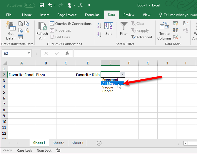
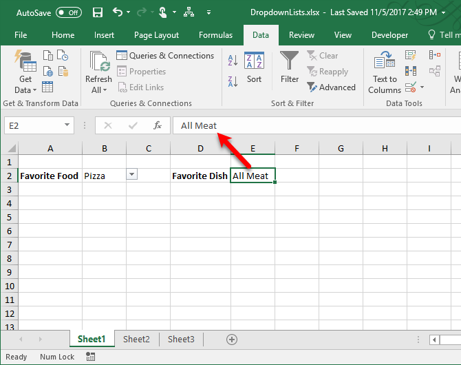
Dropdown lists limit the number of entries for an input field. They help prevent typos and misspellings. And Excel supports surprisingly versatile dropdown list features. Thus, if you want to use Excel for forms or data collection, make it easier for your users to select items with dropdown lists.

Unlock the FREE "Essential Excel Formulas" cheat sheet now!

This will sign you up to our newsletter

Enter your Email

Read our privacy policy

Use a dropdown list in a cell when there are specific options available for that cell. For example, you can create dropdown lists containing options like Male and Female, Yes and No, or any other custom list of options.

We’ll show you how to add dropdown lists to your Excel spreadsheets.

How to Create a Dropdown List in Excel

Creating a dropdown list is easy in Excel, but the process is not obvious. Here is a summary of the steps to create a custom dropdown list in Excel:

1. Create a Named Range: This step is necessary to create the list we’ll be using in your dropdown list.
2. Add Data Validation: This is the not-so-obvious step where you’ll prime the cell for featuring a dropdown list.
3. Add Named Range to Data Validation: Finally, you’ll put it all together and define the source of the dropdown list (i.e. your previously Named Range).
4. Set Input Message for Data Validation: This step is optional. It lets you add a popup message to guide your spreadsheet users.

I love excel enough that even simple data validation + conditional formatting delights me

— x – lily (@ungilded) October 25, 2017

Excel isn’t easy, it’s powerful. This means you have tons of options, as you’ll see shortly. Now let’s look at the steps to making an Excel dropdown list in more detail.

1. Create a Named Range

One way to add a list of items to a dropdown list using Data Validation is to add your list to a worksheet and name the range of cells containing the list. You can add the list to either the same worksheet where you’re going to add the dropdown list or a different worksheet. Using a named range of cells in a dropdown list makes it easier to maintain.

We’re going to create a dropdown list containing some different types of food on Sheet2 as an example. Enter each item in a separate cell either in one column or one row. Select the items, enter a name for the range of selected cells in the Name Box, and press Enter.

2. Add Data Validation

Go to the worksheet where you want to add your dropdown list. Click the Data tab and then click Data Validation in the Data Tools section.

Make sure the Settings tab is active on the Data Validation dialog box.

3. Add Named Range to Data Validation

Then, select List from the Allow dropdown list. We’re going to use the name from the named range of cells we defined to fill the dropdown list. Enter the following text in the Source box.

=Food

Replace “Food” with whatever name you gave your cell range. Click OK.

The Ignore blank checkbox is checked by default. This allows you to select the cell and then deselect the cell without selecting an item. If you want to require an option to be selected from the dropdown list, uncheck the Ignore blank box.

Tom's Tips For Excel: Use Data Validation instead of comment for selected cell: Alt+D+L > Input Message tab > type msg > Ck Show input msg…

— Tom Urtis/Atlas (@TomUrtis) January 22, 2017

4. Set Input Message for Data Validation

If you want a popup message to display when the cell containing the dropdown list is selected, click the Input Message tab. Check the Show input message when the cell is selected box and fill out the Title and Input message boxes. You can also use the Error Alert tab to add a message that displays when invalid input is entered in the dropdown list (e.g. if someone types into the cell rather than selecting an option). Check the Show Error alert after invalid data is entered box. Select a Style and fill out the Title and Error message boxes.

Click OK.

When you select a cell containing a dropdown list, the down arrow for selecting an option displays to the right of the cell. The down arrow button only displays when the cell is selected. We’ll show you a way to display a down arrow next to a dropdown list all the time later in this article.

If the dropdown list contains more than eight items, you’ll see a scroll bar on the dropdown list when you click the arrow.

Advanced Dropdown List Options

Now that you have a basic dropdown list, let’s dive into Excel’s advanced settings for editing and customizing your list.

Edit or Delete a Named Range

If you need to edit or delete a named range, you must use the Name Manager. Click the Formulas tab and then click Name Manager in the Defined Names section.

To change the cell range for a name on the Name Manager dialog box, select the Name in the list and then click the cell range button at the bottom of the dialog box. Then, select the cell range and click the cell range button again on the compact version of the Name Manager dialog box, the same way we described in the section above.

Next, click the green checkmark to save the new cell range for the selected Name.

You can also change a Name by selecting it in the list, clicking Edit, editing the name on the Edit Name dialog box, and clicking OK. You can also change the cell range on the Edit Name dialog box.

To delete a name, select the Name in the list and click Delete.

Create a Dependent Dropdown List

A dependent dropdown list is one in which the options change based on the selection in another dropdown list.

For example, when we select Pizza in the dropdown list we created in the How to Create a Dropdown List section above, a second dependent dropdown list contains the different kinds of pizza. If you select Chinese, the options in the second dependent dropdown list contain different types of Chinese dishes.

Just learned how to create a dependent dropdown list in excel, e.g., cell1-state, cell2-cities in that state. GUYS! It's a life-changer.

— Life at Deloitte (@lifeatdeloitte) February 4, 2014

Before continuing, go back to the How to Create a Dropdown List section and create the main Favorite Food dropdown list, if you haven’t already done so.

Now, we’re going to create three more lists and name them. Enter a list for each of the options in your main dropdown list. Select one of the other lists, enter a name for that list in the Name Box and press Enter. Repeat for each list.

The names of the other lists must match the options in the main dropdown list. For example, one of our other three lists contains types of cookies and is named Cookies, as shown below. The other two lists in the red box on the image below are named Pizza and Chinese.

Before creating the dependent dropdown list, you must select an item in the main dropdown list. It doesn’t matter which option you select. Then, select the cell where you want to add the dependent dropdown list.

Click the Data tab and then click Data Validation in the Data Tools section. Select List in the Allow dropdown list.

Enter the following text in the Source box. Replace “$B$2” with the reference to the cell containing your main dropdown list. Keep the dollar signs in the cell reference. That indicates an absolute reference to the cell that will not change even if you copy or move the formula that references that cell.

=INDIRECT($B$2)

The INDIRECT function returns the reference specified by a text string, in this case, the text from the option selected in the main dropdown list in cell B2. For example, if you select Chinese from the main dropdown list, =INDIRECT($B$2) returns the Chinese reference. As a result, the second dropdown list contains the Chinese items.

Click OK.

The list in the Favorite Dish dropdown list in the example below changes depending on what’s selected in the Favorite Food dropdown list.

Copy and Paste a Dropdown List

If you need to duplicate a dropdown list with data validation to other cells, copy and paste the cell using Ctrl + C and Ctrl + V. This copies the dropdown list and the formatting.

If you just want to copy the dropdown list with the data validation but NOT the formatting, select the cell and copy it normally using Ctrl + C. Then, go to the Home tab and click Paste in the Clipboard section. Select Paste Special.

On the Paste Special dialog box, select Validation in the Paste section. Then, click OK.

This will only copy the dropdown list and not the formatting in the original cell.

Note: Be careful when you are working with dropdown lists in Excel. When you copy a cell that does not contain a dropdown list over a cell that contains a dropdown list, the dropdown list is lost. Excel does not alert you or prompt you for confirmation of the action. However, you can undo the action using Ctrl + Z.

Select All Cells Containing Dropdown Lists

Because the down arrow button does not display on a dropdown list unless that cell is selected, it’s hard to know which cells contain dropdown lists. You could apply different formatting to the cells with dropdown lists. However, you need to find all the dropdown lists first, if you haven’t already formatted them. There is a way to select all cells containing dropdown lists, allowing you to see where they are.

First, select a cell containing a dropdown list. Go to the Home tab and click Find & Select in the Editing section. Then, select Go To Special.

On the Go To Special dialog box, select Data Validation. The All option below Data Validation selects all cells that have any data validation rule applied to it. The Same option only selects cells with dropdown lists using the same type of data validation rule as the one in the selected cell.

We’ll accept the default selection of All because our dropdown lists have slightly different rules. One uses a named range to get its value and the other uses the INDIRECT function.

Click OK.

Our two dropdown lists are selected.

Now you can format these cells to differentiate them from other cells, so you know where all the dropdown lists are. If you would rather not apply different formatting to dropdown lists, the next section shows you another way to make them always visible.

Make the Dropdown List Arrow Always Visible

The down arrow button on a dropdown list goes away when the cell is not selected. We’re going to get around this problem by adding a permanent down arrow button to the right of the dropdown lists.

We took a screenshot of the down arrow button on a dropdown list in Excel. We’re going to insert that image in the cell to the right of the dropdown list, so you see a down arrow button even when the dropdown list is not selected. When selecting the dropdown list, the down arrow button for the list displays over the image we inserted.

To begin, download the drop-down-arrow.png file (right-click on that link and select Save link as). Then, select the cell to the right of a dropdown list and go to the Insert tab.

Then, click Illustrations and select Pictures.

On the Insert Picture dialog box, navigate to where you saved the drop-down-arrow.png file and select the file. Then, click Insert.

The image is inserted on the left side of the cell, looking like it’s connected to the dropdown list in the cell to the left. Now, you know where that dropdown list is, and you can select that cell and the real down arrow button displays over the fake one.

Remove a Dropdown List From a Cell

If you decide you want to remove the dropdown list from a cell, select the cell, and open the Data Validation dialog box as described earlier, in the How to Create a Dropdown List section (go to the Data tab and click Data Validation in the Data Tools section). Click the Clear All button, which is available no matter which tab is currently selected.

The options on the Data Validation dialog box are reset to their defaults. Click OK.

The dropdown list is removed and the cell is restored to its default format. If there was an option selected when you removed the dropdown list, the cell is populated with the value of that option.

If you don’t want any of the values to be preserved when you delete the dropdown list, you can copy a blank cell and pasted it over the cell containing the dropdown list. The dropdown list is removed and the cell becomes a blank cell.

Make Dropdown Lists Work for You

Make full use of dropdown lists for data entry in Excel to be more productive and make your life easier. There are many other form controls available in the Controls section of the Developer tab you can experiment with in your worksheets.

How do you make use of dropdown lists in Excel? Share your thoughts and ideas with us in the comments below. Also, have you mastered Excel charts yet?

Read the full article: How to Create a Dropdown List in Microsoft Excel

Read Full Article

twik.io Personalizes Websites to Increase Conversions

Running a website is fairly easy, but making your visitors happy and having them engage with the site isn’t as easy as you might think. Whether you’re managing content, selling new lines, or promoting the latest initiative, there’s always an issue with engagements.

It might be your site’s tone. Perhaps readers dislike the offer prices, or leave if they don’t feel like the services apply to them. What if you could change this behavior and keep people on your site for longer, with comparatively little effort?

That’s where Automated Personalization platform twik.io comes in. Combining user profiling with objective detection, twik  is a freemium service that matches products and service to users.

What Is an Automated Personalization Platform?

In short, twik AI algorithms automate your personalization delivery on almost every piece of web content (like products, forms, and more) without modifying a single line of code on your site. The team behind twik describes it in the following way:

“The first real-time, fingerprint based, single snippet-installation, fully-automated and GDPR compliant BI, targeting, delivery and personalization engine that increases conversions and retention.”

twik combines user profiling with objective detection to match content to users. So you might want to try out a variety of headlines for a particular product or display different phrases on a call to action (CTA). There’s no single winning variant—every user will get a version of your website that’s twik constantly optimizes for their particular tastes. With these personalized elements, people are more likely to convert.

You’ll manage all this from a visual editor that offers so much control.

How Much Is twik?

twik has a modular pricing structure in place. This makes it attractive to users of all levels, whether you’re a sole website editor or have a network of sites to maintain.

To start, there’s the Freemium option, which covers one domain (additional domains are $20 each). You’ll also get 10,000 pageviews of business intelligence (BI) analysis, 5,000 pageviews of personalization, and a single piece of live content bundled.

Increasing these options means you’ll need to pay. BI comes at $0.001 per pageview, while AI personalization costs $0.002 per pageview.

twik’s unique features are more expensive, however. Live content comes at a cost of $10 per piece, while Pixel queries (which let you check if your visitors are signed into other websites) are $50. However, Pixel queries are only accessible if you add a personal account manager to your plan, which starts at $1,500.

You can adjust your reliance on twik through the useful sliders on the pricing page. Thus, quite simply, you can “pay as you grow.”

Adding twik to Your Website Is Simple

Using twik with your website is remarkably simple. You have three options for integration:

• Place one line of code in the <head> tag, like Google Analytics
• WordPress plugin
• Google Tag Manager

While the one line of code method works if you’re running WordPress, it’s a little more complicated to implement. The plugin works fine; you can grab it from the twik resources page.

twik generates the code for you. Simply log in and add a domain when prompted (or click Domains > + New in the top-left menu), then click Project Settings. Here you’ll find a Snippet ID, along with the HTML/JavaScript code for your site.

While you’re allowed to manage as many domains as you need here, note that twik’s freemium version offers only one domain.

Is twik Breaking Online Privacy Rules?

You’ll also spot the Pixel queries menu in the Project Settings screen. This lets you check if visitors are logged into certain other websites, and is a proprietary technology.

Of course, this begs the question: does twik break online privacy rules?

We’re confident that it doesn’t. A read of the company’s privacy policy should set most minds at rest. As the twik team told us, the service has “no idea who the user is.”

Target Your Audience With twik…

Anyone wishing to target their audience and maximize conversions has various options available with twik. While you might be familiar with similar functionality in Google Analytics, twik goes much deeper by allowing you to target specific demographics through lots of criteria.

Using it, you can reach an individual’s demographic, psychographic, and behavioral data interests such as age, browser, device, gender, geolocation, browsing history, household income (US only), language, network speed, and more. twik can also detect, target, and deliver based on the following factors:

• Device operating system
• Local weather
• New/returning readers
• Open social network in another tab
• The referral URL
• What pages they’ve visited
• Adblock users
• Engagement per session
• Session duration
• Session frequency
• Local currency
• Conversion status
• Whether they’re logged into competitor sites

That’s quite a lot of options—why? As the team described to us:

“Audiences allow you to define user profile groups based on behavioral and demographic KPIs. These, in turn, can be used for targeting/retargeting, experimentation, or BI for specific profile definitions.”

…Then Give Them What They Want

With twik, the aim is to increase conversions and build your audience. Targeting and immediately delivering a tailored customer and user experience to visitors can encourage better actions from carts, forms, posts, and all other actionable elements.

For an online shopping site, that might mean ensuring visitors don’t leave without taking advantage of an offer that’s most suitable for them. A news site might suggest a subscription.

At least, that’s what you should do already. With twik, there’s the opportunity to automate a more aggressive policy of increasing conversions. You can tweak every element on your page, from paragraphs and images to buttons, bars, and headings!

For online shopping, you might target visitors to your store with lower prices than what a competitor offers. If the reader is signed into a fan site or social network page for a certain movie or TV show, you can present them with appropriate piece content on your site.

Consider adding specific content, setting certain specific prices, and even pitching unique offers. To help with this, a Variants Library features “plug and play” scripts free of charge—you can even use the handy Google Ads extension.

Scripts are grouped by Accessibility, Acquisition, Conversion, Engagement, and Retention. These include items like Google Autocomplete for search boxes, Smart Sort Personalization, Social Sharing, automation, and more. It’s also possible to add scripts to the library for sharing with other web personalization advocate worldwide users.

Personalized Automation Increases Conversions

twik.io has the potential to revolutionize how marketers, product managers, C-level executives, site owners, brand advocates, creatives, content editors, and webmasters at every size of organization target their audiences. It lets you deliver nothing but the most interesting and compelling user experience for that customer.

From personalization on titles and buttons to targeting users with uniquely specific backgrounds and activities, twik is a must-have for anyone looking to maximize conversions and make their website more personal for visitors, all through the service’s unique automation.

Even better, what was once an enterprise system is now open to everyone starting for free. Now is the time to get going with twik; head to twik’s homepage and start personalizing your content today.

Image credit: Jirsak/Depositphotos

Read the full article: twik.io Personalizes Websites to Increase Conversions

Read Full Article

12 Ways to Make Your Instagram Stand Out

Instagram is constantly reinventing itself. Which means you need to constantly reinvent yourself as well. With that in mind, here’s how to make your Instagram stand out.

The newest Instagram features offer a lot of opportunities for creativity and individuality, and have brought Instagram back into competition with social media giants like Snapchat.

After years of only using Instagram to upload a single photo at a time, it’s hard for many users to adapt. How do you make a slideshow? Why would you make a Boomerang? What are Instagram stories?

With so many new features available on Instagram, there are more ways than ever to create a unique account. These creative options will help you learn how to make your Instagram stand out.

1. Use Slideshows for “Before and After” Reveals

You aren’t limited to a single photo per post—Instagram offers plenty of different ways to post pictures on Instagram. Using Instagram’s slideshow feature, you can add up to 10 photos, videos, or Boomerangs to a post at one time.

Slideshows are one of the most creative ways to post on Instagram, especially when you post impressive before and after photos to get full shock value. This strategy is effective for new haircuts, repairs, weight loss transformations, sunsets, makeovers, and redecorating.

For a truly dramatic before and after effect, take both photos from the same angle and use the same editing tools on both images.

2. Tell a Story Using Multiple Accounts

View this post on Instagram

Watch EPISODE 2 now on @igorhiller! . YOU RUINED THE PARTY: A 10-part comedy mystery . Directed by @allisonraskin Written by @igorhiller & @allisonraskin . CAST Shannon: @rachelsafety Lisa: @gabyroad Steve: @kunal_d Molly: @rachelretha Rob: @hipablo Patrick: @mj_nelson Bob: @eliolsberg . CREW DP: @dougfrerichs 1st AD/Set Dec: @emmkazz Editor: @jrdnstn Sound: @dominoparker Grip/PA: @eyeswideshutup

A post shared by Allison Raskin (@allisonraskin) on Mar 27, 2017 at 11:00am PDT

Instagram Stories now let you tag other users with a link that goes directly to their accounts. Many Instagram users use this feature to give shoutouts to their favorite accounts.

However, some users are making it worth viewers’ while to click on that link. The video above shows a duo who used their respective audiences to build each other’s follower count.

Over the course of five days, they shared a short film in 10 parts, alternating between each other’s stories. Each part ended on a dramatic cliffhanger, forcing viewers to go to the other’s account if they wanted to see the conclusion.

Even if you don’t have the motivation to make a full short film, try using your Instagram Story effectively by linking it up with a friend. You both build your follower count while providing two different perspectives of the same event—a great method of storytelling.

3. Use Visual Chaining to Keep Your Feed Attractive

When you look at Instagram profiles, some look impossibly perfect. Somehow, every single image seems to coordinate perfectly.

If you want your entire Instagram profile to fit a certain aesthetic or theme, you may want to try something called a “visual chain.” This approach depends on you planning out your photos more than usual, but the overall effect is worth the extra effort.

Every time you post a new photo, think about how it will look next to your previous post and the three before that. Visual chains allow you to get creative with how your profile looks overall. For really impressive effects, try arranging photos by color, content, or photo orientation (as in the example above by @rvstapleton).

4. Use Boomerang to Boost Interest

View this post on Instagram

Sixteen-year-old Dyllon Wolf (@dyllonwolf) coaxed his younger brothers to pop the biggest water balloon of their bunch in our #BoomerangOfTheWeek. “I thought it would remind everyone who saw it of the freedom and joy of being a kid,” Dyllon says. (And he was right.) Follow @boomerangfrominstagram to see more mind-blowing loops from our community. #Boomerang by @dyllonwolf

A post shared by Instagram (@instagram) on Jun 25, 2016 at 10:58am PDT

Boomerangs may seem ridiculous at first glance, but a well-done loop can draw viewers in to your post. The perfect Boomerangs are actions with a distinct beginning and end that look cool when rewound. Some classic Boomerangs are jumping into water, a cool athletic move, traffic, dancing, or a selfie with an exaggerated facial expression.

You can access the Boomerang feature by downloading the Boomerang app for Android or iOS. Or if you press the camera icon in the top left of your screen (typically used to add to your Story), you can create a Boomerang without downloading the app.

Select the Boomerang option at the bottom of the screen, create your video, then save it to your camera roll instead of sending it to your Story. Then, you can upload it to your feed just like you would any other photo or video.

5. Give a Look Behind the Scenes With Slideshow

View this post on Instagram

‘Scavengers’ – an installation using litter, left in Finsbury Park, London, from my first solo show way back in 2008 ?

A post shared by Slinkachu (@slinkachu_official) on Dec 3, 2019 at 11:55pm PST

Instagram user @slinkachu_official creates incredible miniature works of art. However, you don’t truly understand the size or purpose of the artwork until you see a shot of the objects from far away.

The slideshow feature allows viewers to see the “behind the scenes” portions of a finished photo. This approach can add to the Story of how you did something, what led up to the photo, or any other details you think they may find interesting. You can even use videos within a slideshow to add a voice-over explanation of your art or experience.

6. Think Bigger With Giant Square

Try using an app like Giant Square (on iOS and Android), which breaks a single photo into a three-, six-, or nine-square grid. The result makes this method one of the most intriguing ways to make your Instagram stand out.

Keep in mind that each photo still needs to be posted individually to Instagram. That means this option works best with landscape photos, where each individual photo will still look nice on its own.

Selfies, on the other hand, will result in a single photo of your nose being posted inexplicably (especially now that Instagram feeds are algorithm-based instead of chronological). Used correctly, however, this strategy can result in a beautiful and unique Instagram profile (like @photosbywillemthach, seen above).

7. Add Stickers and Drawings to Make Your Story Stand Out

Instagram introduced the stickers and drawings feature in December 2016. This feature initially seemed gimmicky, but it can actually add a lot of fun to your Stories without looking silly.

For example, try adding a thought bubble sticker with custom text. Use several Stories in a row to create a real-life comic strip. Or use the selfie sticker option (pull up stickers after taking your photo or video and then choose the image of your Instagram profile picture). This will let you insert a sticker of your face, which is great for adding visual commentary to a photo of something else.

You can even use stickers to create your own filters. This lets you show off your location or the weather, give people fake accessories, or celebrate holidays. Any emoji you can think of is fair game. Your imagination can truly run wild with this feature.

Don’t forget to add drawings to your Story as well. Quirky drawings and handwritten text can add comedic emphasis to your photo or can point something out. If you don’t know how to draw on Instagram pictures, simply press the squiggly icon at the top of the screen when editing a photo for your Instagram Story.

8. Theme Your Instagram

If you want a solid base of followers, consider giving your Instagram profile a consistent theme. Since Instagram supports multiple accounts, it’s easy to separate your personal posts from your professional or public profile.

Themed Instagrams are far more likely to attract followers, because followers know what types of posts to expect. A well-curated profile allows you to create a consistent Instagram feed and have a beautiful profile with less effort.

Take @muradosmann, for example, who is now world-famous for his Instagram account. His account primarily features photos of his girlfriend leading him around the world, and thousands of global users now use the #FollowMe hashtag.

9. Give Detailed Tutorials Using Every Post Type

Until the introduction of slideshow, Instagram really couldn’t be used for anything content-heavy. But now that multiple images can be added to a single post, complex posts could become the new normal.

For example, try putting together a detailed tutorial using a combination of still images, collages (use Instagram’s Layout app for easy access), video, and text. Simple steps can be a single photo, while more complex steps can have video instructions included. Similarly, use text images for specific instructions or a collage to show a final product comparison.

Tutorials are a great option for Instagram profiles dedicated to cooking, home renovations, makeup routines, or fashion.

10. Use Layout to Create Collages

If you want to add multiple pictures in one post, you don’t always have to create a slideshow. Instead, you can create a collage using Instagram’s Layout app for iOS or Android. Layout allows you to add up to nine different pictures to one collage. This gives you even more different ways to upload photos on Instagram.

After you decide on the pictures, you’ll have to pick out a specific layout. The app offers several different grids to choose from—some have small boxes for your photos, others have large boxes, and then there are those that have a mix of both.

You can rearrange your photos within these boxes, and use Layout’s tools to flip or mirror your photos, as well as add a border. When you’re done, you can post your collage to Instagram just like a typical photo.

11. Post Live Videos to Engage Your Audience

Want to add more personality to your Instagram account? Consider using Instagram Live to post real-time videos. Livestream a video of yourself doing something interesting, or simply take the time to chat with your followers.

When users watch your Instagram Live video, they can submit comments which will immediately appear on the livestream. This makes it easy to relate to your followers or answer any questions. Your video won’t disappear after you turn off the camera, and you can opt to share a replay of your live videos so viewers can catch up later.

12. Still Need Inspiration? Try an Instagram Challenge

If you still feel like you’re struggling to use Instagram creatively, take it back to basics and look at the photos and videos you post. Are you editing your photos carefully? Sometimes third-party Instagram photo editing apps do a better job than Instagram’s native filters and commands.

Next, are your photos interesting and engaging? If you’re having trouble with content, try an Instagram challenge. There are many available online with different goals and lengths depending on your interests.

Some people follow #365Project and post a photo every day of the year. Others participate in smaller challenges (related to yoga, food, the outdoors, or anything you can imagine) led by community leaders from other forms of social media.

You can get involved in challenges by watching the hashtags people you admire use, searching online, or starting your own! Challenges can be a great way to get your creative juices flowing in the middle of a slump and to interact with other users on Instagram.

Learn How to Make Your Instagram Stand Out

You definitely need to take advantage of all the cool ways to post on Instagram. Figuring out how to make your Instagram stand out will make you proud to show off your profile!

For even more Instagram tips and tricks, check out these things you didn’t know you could do on Instagram.

Read the full article: 12 Ways to Make Your Instagram Stand Out

Read Full Article

Got a Windows 10 Wi-Fi Problem? Here’s How to Fix It

When your Windows 10 Wi-Fi is not working, it is one of the most frustrating issues you can encounter. Given that so much of modern computing relies on a web connection, being cut off from the internet can bring your productivity to a screeching halt.

Unlock the FREE "Ultimate Windows Keyboard Shortcuts" cheat sheet now!

This will sign you up to our newsletter

Enter your Email

Read our privacy policy

Keep reading to learn how to fix 10 of the most common Wi-Fi problems on Windows 10.

1. Wi-Fi Is Connected but You Don’t Have internet

Sometimes, Windows will claim you’re connected to the internet and that the connection is secure, but you won’t be able to access the web. Normally, the issue is caused by either a faulty TCP/IP stack, IP address, or DNS client resolver cache.

Firstly, try running Windows’s native Network Troubleshooting tool. You’ll find it in Settings > Update and security > Troubleshoot > internet connections.

If that doesn’t work, open Command Prompt and type the following commands. Press Enter after each command:

• netsh winsock reset
• ipconfig /release
• netsh int ip reset
• ipconfig /renew
• ipconfig /flushdns

If none of that worked, try these tips for the “Connected to Wi-Fi, but no internet” issue.

2. Windows 10 Won’t Connect to Wi-Fi

If you see a message that reads Windows 10 can’t connect to this network while attempting to establish a network connection, your network adapter is probably to blame.

The best solution is to uninstall the network adapter’s driver and allow Windows to reinstall it automatically.

Follow the steps below to complete the process:

1. Press Windows key + X and click on Device Manager.
2. Right-click on the network adapter and choose Uninstall.
3. If prompted, click on Delete the driver software for this device.
4. Restart your machine and Windows will automatically reinstall the driver.

3. Wi-Fi Doesn’t Have a Valid IP Configuration

If you see the Wi-Fi Doesn’t Have a Valid IP Configuration message, you should start by entering the four networking commands we listed earlier.

If the issue persists and your Wi-Fi is still not working on Windows 10, there are two further steps you can take.

Change the Network Name and Password

Some users have reported that simply changing their network’s name and password fixed the problem.

The precise instructions vary between routers, but typically you need to connect to your router using an ethernet cable, enter your router’s IP address in your browser, log into the device’s portal, and locate the correct fields. Make sure you use the right type of Wi-Fi security when you change this info.

Set the Wi-Fi Network’s Channel Width

Without getting too technical, routers can broadcast their networks on different channels. If too many routers in close proximity use the same channel, the airwaves can become cluttered.

Log into your router’s portal and locate the channel setting. If possible, set it to Auto. If there’s no Auto setting, try a few different channels and see if your problem goes away.

4. How to Find Wi-Fi Password on Windows 10

If you’ve bought a new router (or been issued a new one by your ISP), you should always spend the time to change the network’s default name and password. It’s good practice from a security standpoint.

But what if you then forget the password you created? You could reset the router, but there’s a less drastic solution. You can find saved Wi-Fi passwords from within Windows 10.

Just follow the steps below:

1. Right-click on the Network icon on the Taskbar.
2. Choose Open Network internet Settings.
3. In the new window, click on Change adapter options.
4. Right-click on your Wi-Fi connection and select Status.
5. Click on Wireless Properties.
6. Click on the Security tab.
7. Mark the checkbox next to Show Characters.

5. Windows 10 Wi-Fi Driver Issues

We’ve already explained how to delete and reinstall your Wi-Fi driver earlier in the article, but there are a couple of other steps you can also try if you’re having Wi-Fi driver issues on Windows 10. Namely, you can try to either update the Windows 10 driver or roll it back to a previous version.

To update your Wi-Fi driver, follow the steps below:

1. Right-click on the Start Menu.
2. Click on Device Manager.
3. Expand the drop-down menu below Network Adapters.
4. Right-click on your adapter and select Properties.
5. Click on the Driver tab.
6. Choose either Update Driver or Roll Back Driver.

If Windows cannot find an updated driver automatically, you should be able to find it on the manufacturer’s website.

6. No Wi-Fi Networks Found

If your Windows machine cannot find your Wi-Fi network, make some basic troubleshooting checks before moving on. Is the router turned on? Are you within range of the network?

If the answer to both those questions is yes, the next step is to try updating and/or reinstalling the network adapter’s driver. We have already shown you how to do it.

Lastly, you can try changing the region of your Wi-Fi adapter. It’s easy to do, just use the guide below:

1. Press Windows key + R.
2. Type devmgmt.msc and press Enter.
3. Expand the Network Adapters section.
4. Right-click on the name of your network adapter.
5. Choose Properties.
6. Click on the Advanced tab.
7. Highlight Country and Region.
8. Choose the entry according to your location.

Note: Not all network adapters have access to the Country and Region property.

7. Forget Wi-Fi Network on Windows 10

Sometimes, you need your machine to forget a Wi-Fi network. Perhaps you have a new router, or you’re just having a clear out of old networks that you once connected to but no longer use.

Forgetting a Wi-Fi network on Windows 10 is easy:

1. Open the Start Menu and click on Settings.
2. Click on Network and internet.
3. Choose Wi-Fi from the menu on the left-hand side of the screen.
4. Click on Manage known networks.
5. Highlight the name of the network you want to forget.
6. Click on Forget.

8. Windows 10 Keeps Dropping the Wi-Fi Connection

If you find Windows 10 repeatedly drops the Wi-Fi connection without warning (and you’re sure there are no issues with the router), the problem could be caused by your network adapter’s power management settings.

You need to revoke the permission which allows Windows to turn off the adapter to save power. To do so, you’ll once again need to return to the Device Manager:

1. Right-click on the Start Menu and choose Device Manager.
2. Expand the list below Network Adapters.
3. Right-click on your network adapter.
4. Select Properties.
5. Click on the Power Management tab.
6. Unmark the checkbox next to Allow the computer to turn off this device to save power.

9. Your Firewall Prevents Connecting to the Network

Windows comes with a built-in firewall app. It either permits or blocks incoming and outgoing traffic to help protect you against malicious content. However, sometimes, it can block web access for your entire computer.

Obviously, this is not the default behavior. Perhaps you accidentally changed a setting without realizing, or a rogue app overrode your existing rules.

Thankfully, whatever the cause, it’s easy to fix. The solution below works for both the native firewall app as well as any third-party firewall apps you’re running:

1. Open the Start Menu and type Command Prompt.
2. Right-click on the top link and select Run as administrator.
3. Type netsh advfirewall set allprofiles state off and press Enter.
4. Test whether internet access is now working.

To turn your firewalls back on, return to Command Prompt and type netsh advfirewall set allprofiles state on.

10. Your Antivirus Prevents Connecting to the Network

As with the firewall, your anti-virus can also cause connection issues.

You can see which anti-virus apps are installed on your machine by going to the Windows Defender Security Center. You can find it in the list of All Apps on the Start Menu.

When you’ve opened the app, expand the panel on the left-hand side and click Virus and Threat Protection. It will tell you which apps are active and provide you with a shortcut for the app interfaces.

Access the interface of any apps you’re running and temporarily disable the service.

Do You Have Wi-Fi Issues on Windows 10?

In this article, we’ve introduced you to 10 of the most common Wi-Fi issues on Windows 10, then explained some solutions for you to try. Of course, lots of things could go wrong that we’ve not covered.

To learn more about Wi-Fi issues, check out our article on things that might be slowing down your home network.

Read the full article: Got a Windows 10 Wi-Fi Problem? Here’s How to Fix It

Read Full Article