Most of the time, searching an Excel spreadsheet is pretty easy. If you can’t just scan through the rows and columns for it, you can use Ctrl + F to search for it. If you’re working with a really big spreadsheet, it can save a lot of time to use one of these four lookup functions.
Once you know how to search in Excel using lookup, it wont matter how big your spreadsheets get, you’ll always be able to find something in Excel!
1. The VLOOKUP Function
This function allows you to specify a column and a value, and will return a value from the corresponding row of a different column (if that doesn’t make sense, it’ll become clear in a moment). Two examples where you might do this are looking up an employee’s last name by their employee number or finding a phone number by specifying a last name.
Here’s the syntax of the function:
=VLOOKUP([lookup_value], [table_array], [col_index_num], [range_lookup])
- [lookup_value] is the piece of information that you already have. For example, if you need to know what state a city is in, it would be the name of the city.
- [table_array] lets you specify the cells in which the function will look for the lookup and return values. When selecting your range, be sure that the first column included in your array is the one that will include your lookup value!
- [col_index_num] is the number of the column that contains the return value.
- [range_lookup] is an optional argument, and takes 1 or 0. If you enter 1 or omit this argument, the function looks for the value you entered or the next-lowest number. So in the image below, a VLOOKUP looking for an SAT score of 652 will return 646, as it’s the closest number in the list that’s less than 652, and [range_lookup] defaults to 1.
![vlookup-rounding]()
Let’s take a look at how you might use this. This spreadsheet contains ID numbers, first and last names, city, state, and SAT scores. Let’s say you want to find the SAT score of a person with the last name “Winters.” VLOOKUP makes it easy. Here’s the formula you’d use:
=VLOOKUP("Winters", C2:F101, 4, 0)
Because the SAT scores are the fourth column over from the last name column, 4 is the column index argument. Note that when you’re looking for text, setting [range_lookup] to 0 is a good idea. Without it, you can get bad results.
Here’s the result:
![vlookup-excel]()
It returned 651, the SAT score belonging to the student named Kennedy Winters, who is in row 92 (displayed in the inset above). It would’ve taken a lot longer to scroll through looking for the name than it did to quickly type out the syntax!
Notes on VLOOKUP
A few things are good to remember when you’re using VLOOKUP. Make sure that the first column in your range is the one that includes your lookup value. If it’s not in the first column, the function will return incorrect results. If your columns are well organized, this shouldn’t be a problem.
Also, keep in mind is that VLOOKUP will only ever return one value. If you’d used “Georgia” as the lookup value, it would have returned the score of the first student from Georgia, and given no indication that there are in fact two students from Georgia.
2. The HLOOKUP Function
Where VLOOKUP finds corresponding values in another column, HLOOKUP finds corresponding values in a different row. Because it’s usually easiest to scan through column headings until you find the right one and use a filter to find what you’re looking for, HLOOKUP is best used when you have really big spreadsheets or you’re working with values that are organized by time.
Here’s the syntax of the function:
=HLOOKUP([lookup_value], [table_array], [row_index_num], [range_lookup])
- [lookup_value] is the value that you know and want to find a corresponding value for.
- [table_array] is the cells in which you want to search.
- [row_index_num] specifies the row that the return value will come from.
- [range_lookup] is the same as in VLOOKUP, leave it blank to get the nearest value when possible, or enter 0 to only look for exact matches.
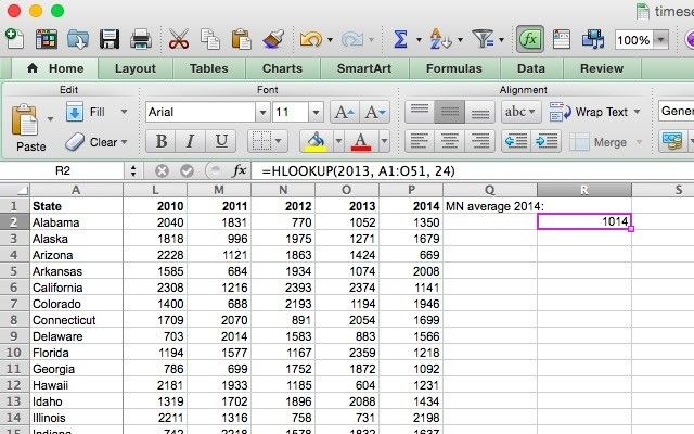
This spreadsheet contains a row for each state, along with an SAT score in the years 2000–2014. You can use HLOOKUP to find the average score in Minnesota in 2013. Here’s how we’ll do it:
=HLOOKUP(2013, A1:P51, 24)
As you can see in the image below, the score is returned:
![hlookup-excel]()
Minnesotans averaged a score of 1014 in 2013. Note that 2013 is not in quotes because it’s a number, and not a string. Also, the 24 comes from Minnesota being in the 24th row.
Notes on HLOOKUP
As with VLOOKUP, the lookup value needs to be in the first row of your table array. This is rarely an issue with HLOOKUP, as you’ll usually be using a column title for a lookup value. HLOOKUP also only returns a single value.
3-4. The INDEX and MATCH Functions
INDEX and MATCH are two different functions, but when they’re used together they can make searching a large spreadsheet a lot faster. Both functions have drawbacks, but by combining them we’ll build on the strengths of both.
First, though, the syntax of both functions:
=INDEX([array], [row_number], [column_number])
- [array] is the array in which you’ll be searching.
- [row_number] and [column_number] can be used to narrow your search (we’ll take a look at that in a moment.)
=MATCH([lookup_value], [lookup_array], [match_type])
- [lookup_value] is a search term that can be a string or a number.
- [lookup_array] is the array in which Microsoft Excel will look for the search term.
- [match_type] is an optional argument that can be 1, 0, or -1. 1 will return the largest value that is smaller than or equal to your search term. 0 will only return your exact term, and -1 will return the smallest value that is greater than or equal to your search term.
It might not be clear how we’re going to use these two functions together, so I’ll lay it out here. MATCH takes a search term and returns a cell reference. In the image below, you can see that in a search for the value 646 in column F, MATCH returns 4.
![match-example]()
INDEX, on the other hand, does the opposite: it takes a cell reference and returns the value in it. You can see here that, when told to return the sixth cell of the City column, INDEX returns “Anchorage,” the value from row 6.
![index-example]()
What we’re going to do is combine the two so that MATCH returns a cell reference and INDEX uses that reference to look up the value in a cell. Let’s say you remember that there was a student whose last name was Waters, and you want to see what this student’s score was. Here’s the formula we’ll use:
=INDEX(F:F, MATCH("Waters", C:C, 0))
You’ll notice that the match type is set to 0 here. When you’re looking for a string, that’s what you’ll want to use. Here’s what we get when we run that function:
![index-match]()
As you can see from the inset, Owen Waters scored 1720, the number that appears when we run the function. This may not seem all that useful when you can just look a few columns over, but imagine how much time you’d save if you had to do it 50 times on a large database spreadsheet that contained several hundred columns!
Let the Excel Searches Begin
Microsoft Excel has a lot of extremely powerful functions for manipulating data, and the four listed above just scratch the surface. Learning how to use them will make your life much easier.
If you really want to master Microsoft Excel, you could really benefit from keeping the Essential Excel Cheat Sheet close to hand!
Image Credit: Cico/Shutterstock
Read the full article: 4 Excel Lookup Functions to Search Spreadsheets Efficiently
Read Full Article
